Artificial Neural Networks: Problems with Multiple Hidden Layers

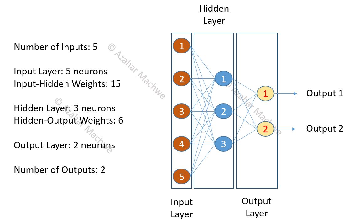
In the last post I described how we work with Multi-layer Perceptron (MLP) model of artificial neural networks. I had also shared my repository on GitHub (https://github.com/amachwe/NeuralNetwork).

I have now added a Single Perceptron (SP) and Multi-class Logistic Regression (MCLR) implementations to it.

The idea is to set the stage for deep learning by showing where these types of ANN models fail and why we need to keep adding more layers.

Single Perceptron:

Let us take a step back from a MLP network to a Single Perceptron to delve a bit deeper into its working.

The Single Perceptron (with a one output) acts as a Simple Linear Classifier. In other words, for a two class problem, it finds a single hyper-plane (n-dimensional plane) that separates the inputs based on their class.


Neural Network Single Perceptron

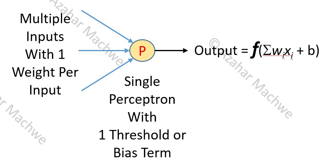
The image above describes the basic operation of the Perceptron. It can have N inputs with each input having a corresponding weight. The Perceptron itself has a bias or threshold term. A weighted sum is taken of all the inputs and the bias is added to this value (a linear model). This value is then put through a function to get the actual output of the Perceptron.

The function is an activation function with the simplest case being the so-called Step Function:

f(x) = 1 if [ Sum(weight * input) + bias ] > 0 

f(x) = -1 if [ Sum(weight*input) + bias ]  <= 0

Perceptron might look simple but it is a powerful model. Implement your own version or walk through my example (rd.neuron.neuron.perceptron.Perceptron) and associated tests on GitHub if you are not convinced.

At the same time not all two-class problems are created equal. As mentioned before, the Single Perceptron partitions the input space using a hyper-plane to provide a classification model. But what if no such separation exists?

Single Perceptron - Linear Separation
Single Perceptron – Linear Separation

The image above represents two very simple test cases: the 2 input AND and XOR logic gates. The two inputs (A and B) can take values of 0 or 1. The single output can similarly take the value of 0 or 1. The colourful lines represents the model which should separate out the two classes of output (0 and 1 – the white and black dots) and allow us to classify incoming data.

For AND the training/test data is:

  • 0, 0 -> 0 (white dot)
  • 0, 1 -> 0 (white dot)
  • 1, 0 -> 0 (white dot)
  • 1, 1 -> 1 (black dot)

We can see it is very easy to draw a single straight line (i.e. a linear model with a single neuron) that separates the two classes (white and black dots), the orange line in the figure above.

For XOR the training/test data is:

  • 0, 0 -> 0 (white dot)
  • 0, 1 -> 1 (black dot)
  • 1, 0 -> 1 (black dot)
  • 1, 1 -> 0 (white dot)

For the XOR it is clear that no single straight line can be drawn that can separate the two classes. Instead what we need are multiple constructs (see figure above). As the single perceptron can only model using a single linear construct it will be impossible for it to classify this case.

If you run a test with the XOR data you will find that the accuracy comes out to be 50%. That might sound good but it is the exact same accuracy if you were to guess one of the classes constantly and the classes were equally distributed. For the XOR case here, as the 0’s and 1’s are equally distributed if we kept guessing 0 or 1 constantly we would still be right 50% of the time.

To put this in contrast to a Multi Layer Perceptron which gives an accuracy of 100%. What is the main difference between a MLP and a Single Perceptron? Obviously the presence of multiple Perceptrons organised in layers! This makes it possible to create models with multiple linear constructs (hyper-planes) which are represented by the blue and green lines in the figure above.

Can you figure out how many units we would need as a minimum for this task? Read on for the answer.

Solving XOR using MLP:

If you used the logic that for the XOR example we need 2 hyper-planes therefore 2 Perceptrons would be required your reasoning would be correct!

Such a MLP network usually would be arranged in a 2 -> 2 -> 1 formation. Where we have two input nodes (as there are 2 inputs A and B), a hidden layer with 2 Perceptrons and a aggregation layer with a single Perceptron to provide a single output (as there is just one output). The input layer doesn’t do anything interesting except presents the values to both the hidden layer Perceptrons. So the main difference between this MLP and a Single Perceptron is that:

  • we add 1 more processing unit (in the hidden layer)
  • to aggregate the output to a single variable an aggregation unit (output layer)

If you check the activation of the individual Perceptrons in the hidden layer (i.e. processing layer) of a MLP trained for XOR you will find a pattern for the activation when presented with type 1 Class (A = B – white dot) and when presented with a type 2 Class (A != B – black dot). One possibility for such a MLP is that:

  • For Class 1 (A = B – white dot): Both the neurons either activate or not (i.e. outputs of the 2 hidden layer Perceptrons are comparable – so either both are high or both are low)
  • For Class 2 (A != B – black dot): The neurons activate asymmetrically (i.e. there is a clear difference between the outputs of the 2 hidden layer Perceptrons)

Conclusions:

Thus there are three takeaways from this post:

a) To classify more complex and real world data which is not linearly separable we need more processing units, these are usually added in the Hidden Layer

b) To feed the processing units (i.e. the Hidden Layer) and to encode the input we utilise an Input Layer which has only one task –  to present the input in a consistent way to the hidden layer, it will not learn or change as the network is trained.

c) To work with multiple Hidden Layer units and to encode the output properly we need an aggregation layer to collect output of the Hidden Layer, this aggregation layer is also called an Output Layer


I would again like to bring up the point of input representation and encoding of output:

  • We have to be careful in choosing the right input and output encoding
  • For the XOR and other logic gate example we can simply map the number of bits to the number of inputs/outputs but what if we were trying to process handwritten documents – would you have one character per output? How would you organise the inputs given that the handwritten data can be of different length?

In the next post we will start talking about Deep Learning as we have provided two very important reasons for so-called shallow networks to fail.

Artificial Neural Networks: An Introduction

Artificial Neural networks (ANNs) are back in town after a rather long exile to the edges of Artificial Intelligence (AI) product space. Therefore I thought I would do a post on it to provide an introduction.

For a one line intro: An Artificial Neural Network is a Machine Learning paradigm that mimics the structure of the human brain.

Some of the biggest tech companies in the world (i.e. Google, Microsoft and IBM) are investing heavily in ANN research and in creating new AI products such as driver-less cars, language translation software and virtual assistants (e.g. Siri and Cortana).

There are three main reasons for a resurgence in ANNs:

  1. Availability of cheap computing power in form of multi-core CPUs and GPUs which enables machines to process and learn from ‘big-data’ using increasingly sophisticated networks (e.g. deep learning networks)
  2. Problem with using existing Machine Learning methods against high volume data with complex representations (e.g. images, videos and sound) required for novel applications such as driver-less cars and virtual assistants
  3. Availability of free/open source general  purpose ANN libraries for major programming languages (i.e. TensorFlow/Theano – Python; DL4J – Java), earlier either you had to code ANNs from scratch or shell out money for specialised software (e.g. Matlab plugins)

My aim is to provide a trail up to the current state of the art (Deep Learning) over the space of 3-4 posts. To start with, in this post I will talk about the simplest form of ANN (also one of the oldest), called a Multi-Layer Perceptron Neural Network (MLP).

Application Use-Case:

We are going to investigate a supervised learning classification task using simple MLP networks with a single hidden layer, trained using back-propagation.

Simple Multi-Layer Perceptron Network:

MLP Neural Network
Neural Network (MLP)

The image above describes a simple MLP neural network with 5 neurons in the input layer, 3 in the hidden layer and 2 in the output layer.

Data Set for Training ANNs:

For supervised learning classification tasks we need labelled data sets. Think of it as a set of input – expected output pairs. The input can be an image, video, sound clip, sensor readings etc.; the label(s) can be set of tags, words, classes, expected state etc.

The important thing to understand is that whatever the input, we need to define a representation that optimally describes the features of interest that will help with the classification.

Representation and feature identification is a very important task that machines find difficult to do. For a brain that has developed normally this is a trivial task. Because this is a very important point I want to get into the details (part of my Ph.D. was on this topic as well!).

Let us assume we have a set of grey scale images as the input with labels against them to describe the main subject of the image. To keep it simple let us also assume a one-to-one mapping between images and tags (one tag per image). Now there are several ways of representing these images. One option is to flatten each image into an array where each element represents the grey scale value of a pixel. Another option is to take an average of 2 pixels and take that as an array element. Yet another option is to chop the image into fixed number of squares and take the average of that. But the one thing to keep in mind is whatever representation we use, it should not hide features of importance. For example if there are features that are at the level of individual pixels and we use averaging representation then we might loose a lot of information.

The labels (if less in number) can be encoded using binary notation otherwise we can use other representations such as word vectors.

To formalise:

If is a given input at the Input Layer;

is the expected output at the Output Layer;

Y’ is the actual output at the Output Layer;

Then  our aim is to learn a model (M) such that:

Y’ = M(X) where Error calculated by comparing and Y’ is minimised.

One method of calculating Error is (Y’-Y)^2

To calculate the total error for training examples me just use the Mean Squared Error formula (https://en.wikipedia.org/wiki/Mean_squared_error)

Working of a Network:

The MLP works on the principle of value propagation through different layers till it is presented as an ouput at the output layer. For a three layer network the propagation of value is as follows:

Input -> Hidden -> Output -> Actual Output

The propagation of the Error is in reverse.

Error at Output -> Output -> Hidden -> Input

When we propagate the Error back through the network we adjust the weights and biases between the Output-Hidden and Hidden-Input layers. The adjustment is carried out one layer at a time keeping all other layers the same (i.e. updates are applied to the entire network in a single step). This process is called ‘Back-propagation’. The idea is to minimise the Error which is computed as a ‘gradient descent’, sort of like walking through a hilly region but always down hill. What gradient descent does not guarantee is whether the lowest point (i.e. Error) you will reach will be the Global Minimum – i.e. there are no guarantees that the lowest Error figure you found is the lowest possible Error figure unless the error is zero!

This excellent post describes the process of ‘Back-propagation’ in detail with a worked example: https://mattmazur.com/2015/03/17/a-step-by-step-backpropagation-example/

The one key point of the process is that as we move from Output to the Input layer, tweaking the weights as we perform gradient descent, a chain of interactions is formed (e.g. Input Neuron 1 affects all Hidden Neurons which in turn affect all Output Neurons). This chain becomes more volatile as the number of Hidden Layers increase (e.g. Input Neuron 1 affects all Hidden Layer 1 Neurons which affect all Hidden Layer 2 Neurons … which affect all Hidden Layer M Neurons which affect all the Output Neurons). As we go deeper into the network the effect of individual hidden neurons on the final Error at the output layer becomes small.

This leads to the problem of the ‘Vanishing Gradient’ which limits the use of traditional methods for learning when using ‘deep’ topologies (i..e. more than 1 hidden layer) because this chained adjustment to the weights becomes unstable and for deeper layers the process no longer resembles following a downhill path. The gradient can become insignificant very quickly or it can become very large.

When training all training examples are presented one at a time. For each of the examples the network is adjusted (gradient descent). Each loop through the FULL set of training examples is called an epoch.

The problem here can be if there are very large number of training examples and their presentation order does not change. This is because initial examples lead to larger change in the network.So if the first 10 examples (say) are similar, then the network will be very efficient at classifying those class of cases but will generalise to other classes very poorly.

A variation of this is called stochastic gradient descent where training examples are randomly selected so the danger of premature convergence is reduced.

Working of a Single Neuron:

A single neuron in a MLP network works by combining the input it receives through all the connections with the previous layer, weighted by the connection weight; adding an offset (bias) value and putting the result through an activation function.

  1. For each input connection we calculate the weighted value (w*x)
  2. Sum it across all inputs to the neuron (sum(w*x))
  3. Apply bias (sum(w*x)+bias)
  4. Apply activation function and obtain actual output (Output = f( sum(w*x)+bias ))
  5. Present the output value to all the neurons connected to this one in the next layer

When we look at the collective interactions between layers the above equations become Matrix Equations. Therefore value propagation is nothing but Matrix multiplications and summations.

Activation functions introduce non-linearity into an otherwise linear process (see Step 3 and 4). This allows the network to handle non-trivial problems. Two common activation functions are: Sigmoid Function and Step Function.

More info here: https://en.wikipedia.org/wiki/Activation_function

Implementation:

I wanted to dig deep into the workings of ANNs which is difficult if you use a library like DL4J. So I implemented my own using just JBLAS matrix libraries for the Matrix calculations.

The code can be found here: https://github.com/amachwe/NeuralNetwork

It also has two examples that can be used to evaluate the working.

  1. XOR Gate
    1. Has 4 training instances with 2 inputs and a single output, the instances are: {0,0} -> 0; {1,1} -> 0; {1,0} -> 1; {0,1} -> 1;
  2. MNIST Handwritten Numbers
    1. Has two sets of instances (single handwritten digits as images of constant size with corresponding labels) – 60k set and 10k set
    2. Data can be downloaded here: http://yann.lecun.com/exdb/mnist/

MNIST Example:

The MNIST dataset is one of the most common ‘test’ problems one can find. The data set is both interesting and relevant. It consists of images of hand written numbers with corresponding labels. All the images are 28×28 and each image has a single digit in it.

We use the 10k instances to train and 60k to evaluate. Stochastic Gradient Descent is used to train a MLP with a single hidden layer. The Sigmoid activation function is used throughout.

The input representation is simply a flattened array of pixels with normalised values (between 0 and 1). A 28×28 image results in an array of 784 values. Thus the input layer has 784 neurons.

The output has to be a label value between 0 and 9 (as images have only single digits). We encoded this by having 10 output neurons with each neuron representing one digit label.

That just leaves us with the number of hidden neurons. We can try all kinds of values and measure the accuracy to decide what suits best. In general the performance will improve as we add more hidden units up to a point after that we will encounter the law of diminishing returns. Also remember more hidden units means longer it takes to train as the size of our weight matrices explode.

For 15 hidden units:

  • a total of 11,760 weights have to be learnt between the input and hidden layer 
  • a total of 150 weights have to be learnt between the hidden and output layer

For 100 hidden units:

  • a total of 78,400 weights have to be learnt between the input and hidden layer
  • a total of 1000 weights have to be learnt between the hidden and output layer
Hidden Units and performance
Hidden Units and Performance

The graph above shows what happens to performance as the number of hidden layer units (neurons) are increased. Initially from 15 till about 100 decent performance gains are achieved at the expense of increased processing time. But after 100 units the performance increase slows down dramatically. Fixed learning rate of 0.05 is used. The SGD is based on single example (mini-batch size = 1)

Vanishing Gradient in MNIST:

Remember the problem of vanishing gradient? Let us see if we can highlight its effect using MNIST. The chaining here is not so bad because there is a single hidden layer but still we should expect the outer – hidden layer weights to have on average larger step size when the weights are being adjusted as compared to the inner – hidden layer weights (as the chain goes from output -> hidden -> input). Let us try and visualise this by sampling the delta (adjustment) being made to weights along with which layer they are in and how many training examples have been shown.

weights update by layer
Weights update by layer and number of training examples

After collecting millions of samples (remember for a 100 hidden unit network each training instance results in almost 80,000 weight updates so it doesn’t take long to collect millions of samples) of delta weight values in hidden and input layer we can take their average by grouping based on layer and stage of learning to see if there is significant difference in the step sizes.

What we find (see image above) is as expected. The delta weight updates in the outer layer are much higher than in the hidden layer to start with, but it converges rapidly as more training examples are presented.Thus the first 250 training examples have the most effect.

If we had multiple hidden layers, the chances are that delta updates for deeper layers would be negligible (maybe even zero). Thus the adaption or learning is being limited to the outer layer and the hidden layer just before it. This is called shallow learning. As we shall see to train multiple hidden layers we have to use a divide and rule strategy as compared to our current layer by layer strategy.

Keep this in mind as in our next post we will talk about transitioning from shallow to deep networks and examine the reasons behind this shift.