October 2016 – Fish Eye View

Artificial Neural Networks: Training for Deep Learning – IIb

This post, like the series provides a pathway into deep learning by introducing some of the concepts using some common reference points. This is not designed to be an exhaustive research review of deep learning techniques. I have also tried to keep the description neutral of any programming language, though the backing code is written in Java.

So far we have visited shallow neural networks and their building blocks (post 1), investigated their performance on difficult problems and explored their limitations (post 2). Then we jumped into the world of deep networks and described the concept behind them (post 3) and the RBM building block (post 4). Then we started discussing a possible local (greedy) training method for such deep networks (post 5). In the previous post we started talking about the global training and also about the two possible ‘modes’ of operation (discriminative and generative).

In the previous post the difference between the two modes was made clear. Now we can talk a bit more about how the global training works.

As you might have guessed the two operating modes need two different approaches to global training. The differences in flow for the two modes and the required outputs also means there will be structural differences when in the two modes as well.

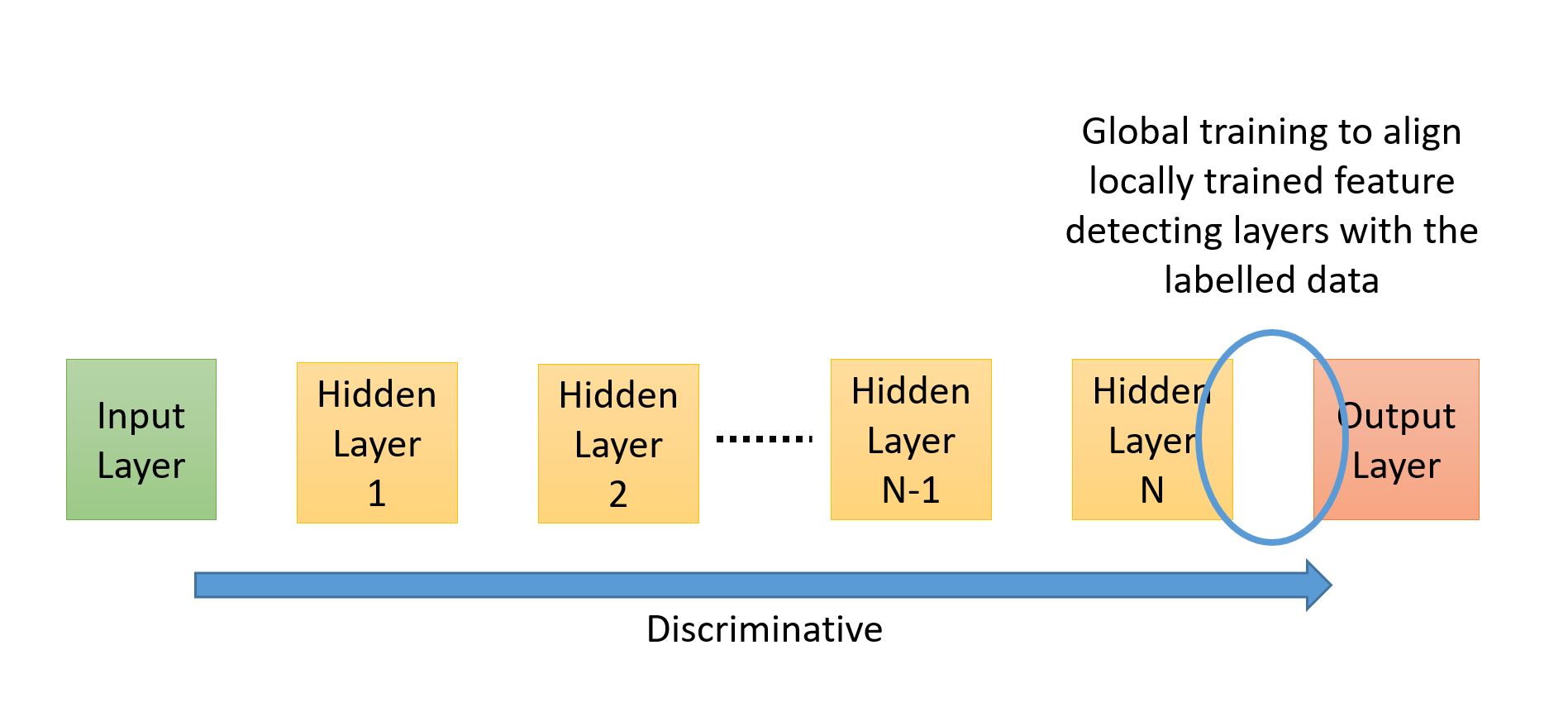
The image below shows a standard discriminative network where flow of propagation is from input to the output layer. In such networks the standard back-propagation algorithm can be used to do the learning closer to the output layers. More about this in a bit.

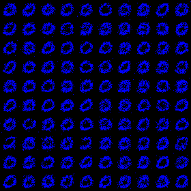
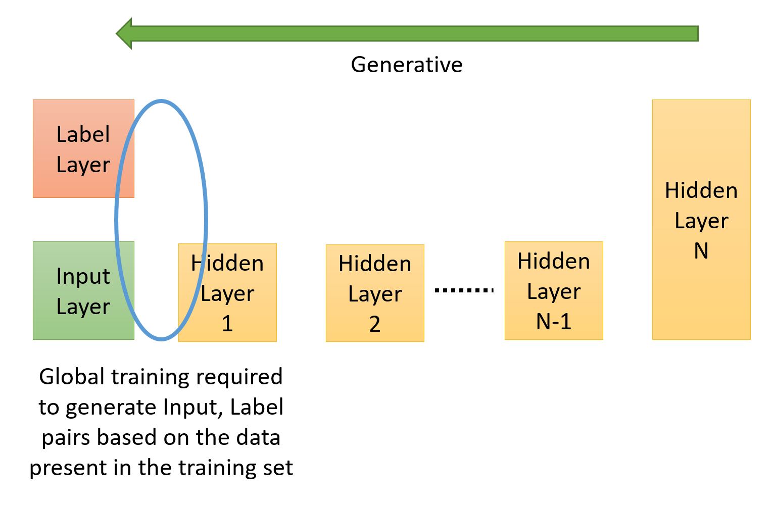
The image below shows a generative network where the flow is from the hidden layers to the visible layers. The target is to generate an input, label pair. This network needs to learn to associate the labels with inputs. The final hidden layer is usually lot larger as it needs to learn the joint probability of the label and input. One of the algorithms used for global training of such networks is called the ‘wake-sleep’ algorithm. We will briefly discuss this next.

Wake-Sleep Algorithm:

The basic idea behind the wake-sleep algorithm is that we have two sets of weights between each layer – one to propagate in the Input => Hidden direction (so called discriminative weights) and the other to propagate in the reverse direction (Hidden => Input – so called generative weights). The propagation and training are always in opposite directions.

The central assumption behind wake-sleep is that hidden units are independent of each other – which holds true for Restricted Boltzmann Machines as there are no intra-layer connections between hidden units.

Then the algorithm proceeds in two phases:

Wake Phase: Drive the system using input data from the training set and the discriminative weights (Input => Hidden). We learn (tune) the generative weights (Hidden => Input) – thus we are trying to learn how to recreate the inputs by tuning the generative weights
Sleep Phase: Drive the system using a random data vector at the top most hidden layer and the generative weights (Hidden => Input). We learn (tune) the discriminative weights (Input => Hidden) – thus we are trying to learn how to recreate the hidden states by tuning the discriminative weights

As our primary target is to understand how deep learning networks can be used to classify data we are not going to get into details of wake-sleep.

There are some excellent papers for Wake-Sleep by Hinton et. al. that you can read to further your knowledge. I would suggest you start with this one and the references contained in it.

Back-propagation:

You might be wondering why we are talking about back-prop (BP) again when we listed all those ‘problems’ with it and ‘deep networks’. Won’t we be affected by issues such as ‘vanishing gradients’ and being trapped in sub-optimal local minima?

The trick here is that we do the pre-training before BP which ensures that we are tuning all the layers (in a local – greedy way) and giving BP a head start by not using randomly initialised weights. Once we start BP we don’t care if the layers closer to the input layer do not change their weights that much because we have already ‘pointed’ them in a sensible direction.

What we do care about is that the features closer to the output layer get associated with the right label and we know BP for those outer layers will work.

The issue of sub-optimal local minima is addressed by the pre-training and the stochastic nature of the networks. This means that there is no hard convergence early on and the network can ‘jump’ its way out of a sub-optimal local minima (with decreasing probability though as the training proceeds).

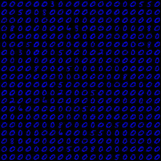
Classification Example – MNIST:

The easiest way to go about this is to use ‘shallow’ back propagation where we put a layer of logistic units on top of the existing deep network of hidden units (i.e. the Output Layer in the discriminative arrangement) and only this top layer is trained. The number of logistic units is equal to the number of classes we have in the classification task if using one-hot encoding to encode the classes.

An example is provided on my github, the test file is: rd.neuron.neuron.test.TestRBMMNISTRecipeClassifier

This may not give record breaking accuracy but it is a good way of testing discriminative deep networks. It also takes less time to train as we are splitting the training into two stages and always ever training one layer at a time:

Greedy training of the hidden layers
Back-prop training of the output layer

The other advantage this arrangement has is that it is easy to reason about. In stage 1 we train the feature extractors and in stage 2 we train the feature – class associations.

One example network for MNIST is:

Input Image > 784 > 484 > 484 > 484 > 10 > Output Class

This has 3 RBM based Hidden Layers with 484 neurons per layer and a 10 unit wide Logistic Output Layer (we can also use a SoftMax layer). The Hidden Layers are trained using CD10 and the Output Layer is trained using back propagation.

To evaluate we do peak matching – the index of the highest value at the output layer must match the one-hot encoded label index. So if the label vector is [0, 0, 0, 1, 0, 0, 0, 0, 0, 0] then the index value for the peak is 3 (we use index starting at 0). If in the output layer the 4th neuron has the highest activation value out of the 10 then we can say it detected the right digit.

Using such a method we can easily get an accuracy of upwards of 95%. While this is not a phenomenal result (the state of the art full network back-prop gives > 99% accuracy for MNIST), it does prove the concept of a discriminative deep network.

The trained model that results is: network.discrm.25.nw and can be found on my github here. The model is simply a list of network layers (LayerIf).

The model can be loaded using:

[codesyntax lang=”java5″]

List<LayerIf> network = StochasticNetwork.load(fileName);

[/codesyntax]

You can use the Propagate class to use it to ‘predict’ the label.

The PatternBuilder class can be used to measure the performance in two ways:

Match Score: Matches the peak index of the one-hot encoded label vector from the test data with the generated label vector. It is a successful match (100%) is the peaks in the two vectors have the same indexes. This does not tell us much about the ‘quality’ of the assigned label because our ‘peak’ value could just be slightly bigger than other values (more of a speed breaker on the road than a peak!) as long as it is strictly the ‘largest’ value. For example this would be a successful match:
1. Test Data Label: [0, 0, 1, 0] => Actual Label: [0.10, 0.09, 0.11, 0.10] as the peak indexes are the same ( = 2 for zero indexed vector)
2. and this would be an unsuccessful one: Test Data Label: [0, 0, 1, 0] => Actual Label: [0.10, 0.09, 0.10, 0.11] as the peak indexes are not the same
Score: Also includes the quality aspect by measuring how close the Test Data and Actual Label values are to each other. This measure of closeness is controlled by a threshold which can be set by the user and incorporates ALL the values in the vector. For example if the threshold is set to 0.1 then:
1. Test Data Label: [0, 0, 1, 0] => Actual Label: [0.09, 0.09, 0.12, 0.11] the score will be 2 out of 4 (or 50%) as the last index is not within the threshold of 0.1 as | 0 – 0.11 | = 0.11 which is > 0.1 and same with | 1 – 0.12 | = 0.88 which is > 0.1 thus we score them both a 0. All other values are within the threshold so we score +1 for them. In this case the Match Score would have given a score of 100%.

Next Steps:

So far we have just taken a short stroll at the edge of the Deep Learning forest. We have not really looked at different types of deep learning configurations (such as convolution networks, recurrent networks and hybrid networks) nor have we looked at other computational models of the brain (such as integrate and fire models).

One more thing that we have not discussed so far is how can we incorporate the independent nature of neurons. If you think about it, the neurons in our brains are not arranged neatly in layers with a repeating pattern of inter-layer connections. Neither are they synchronized like in our ANN examples where all the neurons in a layer were guaranteed to process input and decide their output state at the SAME time. What if we were to add a time element to this? What would happen if certain neurons changed state even as we are examining the output? In other words what would happen if the network state also became a function of time (along with the inputs, weights and biases)?

In my future posts I will move to a proper framework (most probably DL4J – deep learning for java or TensorFlow) and show how different types of networks work. I can spend time and implement each type of network but with a host of high quality deep learning libraries available, I believe one should not try and ‘reinvent the wheel’.

If you have found these blog posts useful or have found any mistakes please do comment! My human neural network (i.e. the brain!) is always being trained!

Artificial Neural Networks: Training for Deep Learning – IIa

This is the second post on Training a Deep Learning network. The best way to read through is by starting from the first post (see above).

So far we have visited shallow neural networks and their building blocks (post 1), investigated their performance on difficult problems and explored their limitations (post 2). Then we jumped into the world of deep networks and described the concept behind them (post 3) and the RBM building block (post 4). Finally in the previous post we started describing a possible training method for such deep networks (post 5) where we take a local view of the network..

In this post we describe the other side of the training process – where we take the global view of the network.

Network Usage:

Before we start that though, it is very important to take a step back and review what we are trying to do.

Our target is to train a neural network that can be used to classify complex data to a high degree of accuracy for tasks that are relatively easy for Humans to do.

Classification can be done in one of two ways: Discriminative or Generative. We have touched on these in the previous post as well. From a practical perspective the choice needs to be made on the basis of what we want our network to do. If we want to use it for a purely label generation task for an input then it is enough to have a discriminative model (which basically calculates p (label | input)). Here we are attempting to assign a label to a set of features extracted from the input. That is why discrimintative training requires labelled training data.

If you want to actually create new inputs based on certain features then you need to have a generative model (which calculates p (label , input)). In case of a generative model we do not ‘discriminate’ between inputs based on features using labels (i.e. try and find the label/class boundary). Instead we treat them as a pair of variables and we try and model their joint probability. This allows us to create new pairs of inputs and features based on the learned joint probabilities.

For example: if we are using MNIST just to recognise and label handwritten digits then we can work with a discriminative model. To get the discriminative output we need some sort of a ‘capping’ output layer (e.g. softmax) which gives us one clear label (for this example there is one to one correspondence between input and label). We cannot directly work with a probability distribution of features (similar to what we saw in the last post) as an output. The process here is inherently one way, present an input and get the label as an output (thus the propagation is away from the input layer).

But what if we wanted to generate new ‘handwritten’ digits (think of an app that translates a typed letter into a handwritten one which matches your handwriting!). If we learn p(input , label) we can easily reverse it as we could start with a label and get an ‘input’ (hand written digit). The direction of generative propagation is opposite to the discriminative one (the propagation is towards the input layer).

Does this mean that we should always target a generative model as it gives us more flexibility? The short answer is No, because generative models usually have poor performance as compared to their discriminative cousins. The long answer is ‘depends on the use-case’.

Symbol Grounding Problem:

Another reason why we show special interest in generative models is because the standard ‘data’ labeling process is very artificial. In real life no such clear labels exist for most of what we experience or even worse: there may be too many labels. For example if we show an image of a cartoon car to say 10 different people and ask them to assign one label to it we are more than likely to get multiple labels such as: cartoon car, car, cartoon… and that is just in the English language! If we had people in that group whose first language was not English they might use other labels which may or may not have a direct correlation with the corresponding English language labels. In fact all these labels are just different symbols that assign meaning to the data. This is the ‘symbol grounding problem’ in AI.

Our brain definitely does not work with strict labels. In fact it matches the joint distribution behavior better – the cartoon in the above example can be analysed at different levels such as: a cartoon, a cartoon car, a cartoon sports car, a cartoon sports car driving very fast…. so as we analyse the same input we have a growing set of labels associated with it.

It would be very messy if we had to learn a different discriminative model for each of the associated labels that operates on the same input data. Also it would be impossible if we were asked to draw a cartoon sports car without some kind of generative model that takes into account all its possible ‘characteristics’ and returns a learned representation (shape, components, size etc.).

If we also take a look at human cognition (which is what we are trying to mimic) simple classification is just one half of the process. Without the generative ability we would not be able to react to the result of the classification. Our brain may classify the weather as ‘likely to be wet’ as the image of the sky travels from the eye to the brain, but it is the reverse propagation from the brain to our muscles that ensures we pick up the umbrella.For our example: As our brain classifies and breaks down the task of drawing a cartoon sports car it needs to switch into generative mode to actually draw it out.

Here we also have a good reason why generative models should NOT be very accurate or rigid. If we had rigidly learnt generative models that did not change over time (or were very difficult to re-train), there would be no concept of ‘training’, ‘skill’ or ‘creativity’. Given a set of features we all would produce the same (or similar) cartoon sports car! There would be very little difference between the cartoon sports car drawn by a professional cartoonist and one drawn by a child as after a certain point in time a rigid generative model would not respond to additional training.

Note: the above description is an over-simplification of some very complex cognitive processes and is intended only as an aid in understanding the concepts being presented in this post.

MNIST Example:

We can generate digits as we learn to classify them using the greedy learning algorithm described in the previous post. This can be done by simply reversing the direction of propagation from Input => Hidden to Hidden => Input and doing some sampling using clamped hidden vectors.

The process is very simple:

Randomly generate a binary vector equal in length to the top most hidden layer
Clamp this vector to the hidden layer and then propagate down to the visible and back up to the hidden ‘n’ number of times (thus feeding back the result at both hidden and visible layers)
For the last iteration do not propagate back to the hidden unit instead convert the vector on the visible layer into an image

For the test we have the standard MNIST input layer (28 x 28 = 784 inputs). Following that we have 3 hidden layers of 100 neurons each. Each hidden layer is trained using CD-10 on a mini batch of the MNIST dataset. I will be uploading the associated test files on my github. The file is: rd.neuron.neuron.test.TestRBMMNISTRecipe

When we set n = 0 we get very fuzzy generated digits:

I can make out a few rough 2s and a some half formed digits and a lot of ‘0’s!

Let us set n = 5 (therefore we do down – up for 5 times and then the 6th pass is just down):

As you can see the generated digits are a lot cleaner and we also have some relatively complicated digits (‘3’ and ‘6’) and a rough ‘8’ (3rd row from bottom, 4th column from right).

This proves that our network has learnt the features associated with handwritten digits which it uses to generate new data.

As a final example, let us set n = 50 and generate a larger set of digits:

In the next post we delve deeper into the ‘feature’ – ‘label’ training process and show how we can get our deep network to classify hand-written digits.