DBSCAN is quite an old algorithm, being proposed in 1996 [1]. But that doesn’t make it any less exciting. Unlike K-Means Clustering, in DBSCAN we do not need to provide the number of clusters as a parameter as it is ‘density’-based. What we provide instead are: size of the neighbourhood (epsilon – based on a distance metric) and minimum number of points to form a dense region (including the point being examined).
Minimum Number of Points: this is usually the dimensionality of the data + 1. If this is a large number we will find it difficult to designate a dense region.
Epsilon – Neighbourhood Size: this should be chosen keeping in mind that a high value will tend to group regions together into large clusters and a low value will result in no clustering at all.
The algorithm attempts to sort a dataset into either a noise point (an outlier – not in any cluster) or a cluster member.
Walking through the DBSCAN Algorithm
I will walk through the algorithm linking it with specific code segments from: https://github.com/amachwe/db_scan/blob/main/cluster.py. Figure 1 shows some data points in 2d space. Assume minimum number of points is 3 (2d + 1).

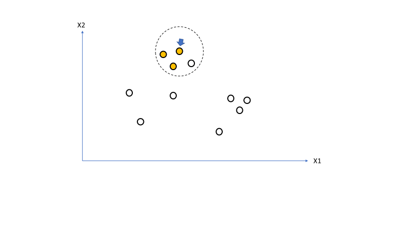
First loop of the iteration we select a point and identify its neighbourhood [line 31]. From Figure 2 we see 3 points in the neighbourhood therefore the point being examined is not a noise point [line 33]. We can therefore assign the point to a cluster (orange) [line 37].
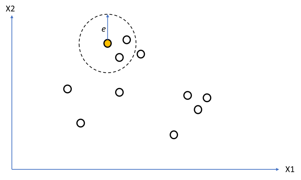
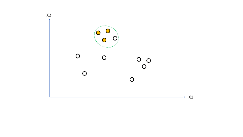
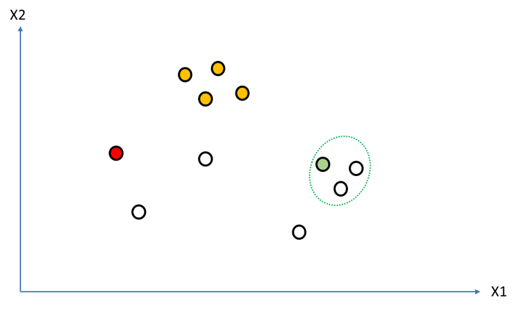
Figure 3 shows the seed set for the point being examined [lines 38-40] as the green dotted line.

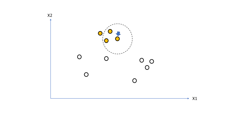
We take the first point in the seed set (marked by the blue arrow) [line 40] and mark it as a point belonging the current cluster (orange) [line 48] then we identify its neighbourhood [line 49]. This is shown in Figure 4.
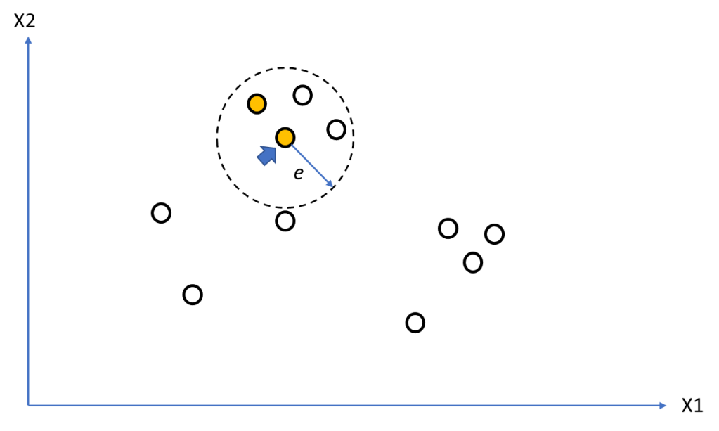
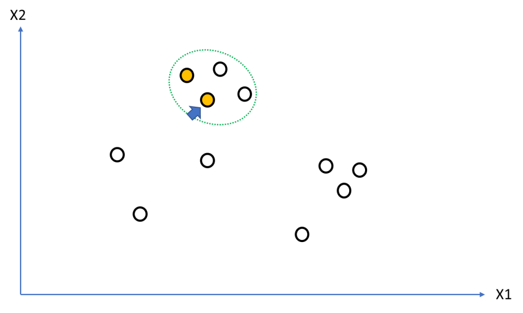
Figure 5 shows the expanded seed set [lines 51-56] because of the new neighbourhood of the current seed set point being examined.
We keep repeating the process till all points in the seed set are processed (Figure 6-8) [lines 40-56]. Even though the seed set contains the first point we started with, when it is processed line 44 checks if the point being checked has already been assigned to a cluster.
Noise Points
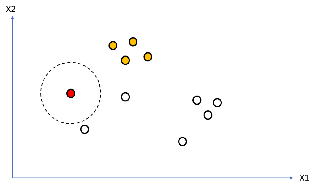
Figure 9 shows the state after first four points have been processed and have been identified to belong to a cluster (orange). Now we get a point that we can visually confirm is an outlier. But we need to understand how the algorithm deals with it. We can see the selected point (red) has no neighbours within distance e. Therefore the condition on line 33 will kick in and this point will be identified as a noise point.
The algorithm continues to the next point (see Figure 10) after incrementing the cluster label [line 58] and starts a new cluster (green). We again identify its neighbourhood points and create a new seed set (Figure 11)

Testing
Testing script (Python Notebook) can be found here: https://github.com/amachwe/db_scan/blob/main/cluster_test.ipynb
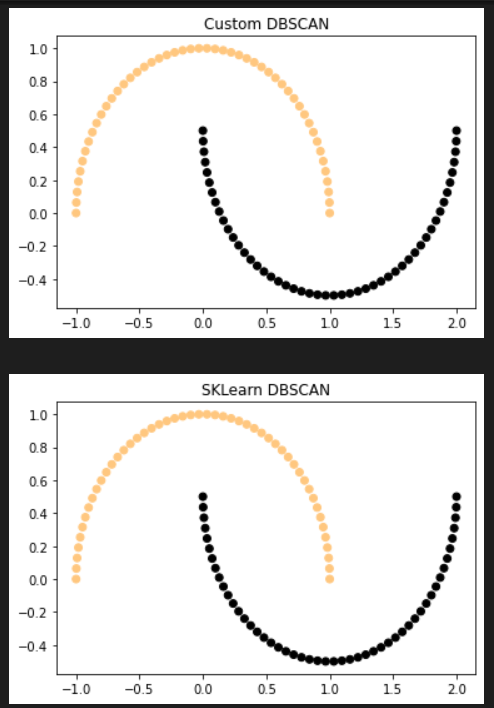
The first block contains some data generation functions – a combination of commonplace ones such as Iris and Make Moons as well as some custom ones.
Make Moons Function
No noise points. Number of Clusters: 2.
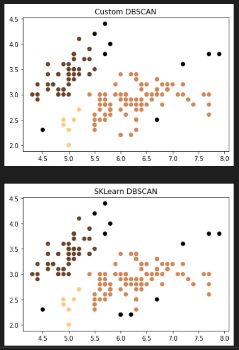
Iris Dataset
Noise match (%): 85.71 between algorithms. Number of clusters: 3.