ADK 2.0 is officially out. Being moved from preview to GA in record time by Google. And of course I have to take it for a spin especially as v2.0 is expected to plug some big gaps between the control and simplicity of LangChain/LangGraph and the abstraction and speed of development of ADK.
But before we dive in couple of things to remember:
- ADK v1.0 took abstraction as the approach to provide speed of development therefore, it has to peel back the hood to provide greater flow control.
- It is always more difficult to decrease abstraction than increase it (point in evidence the move of LangChain to LangGraph to out of the box agents to now ‘deep agents’).
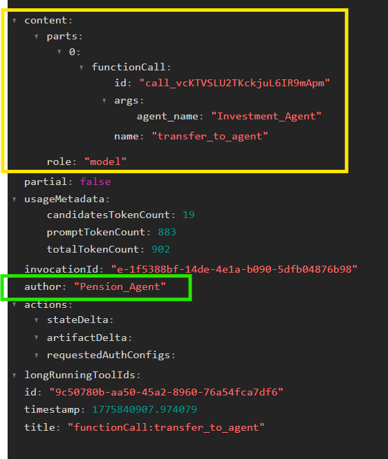
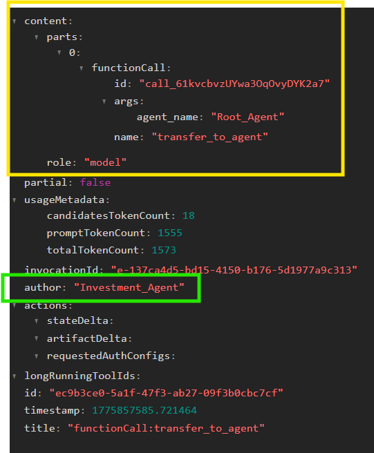
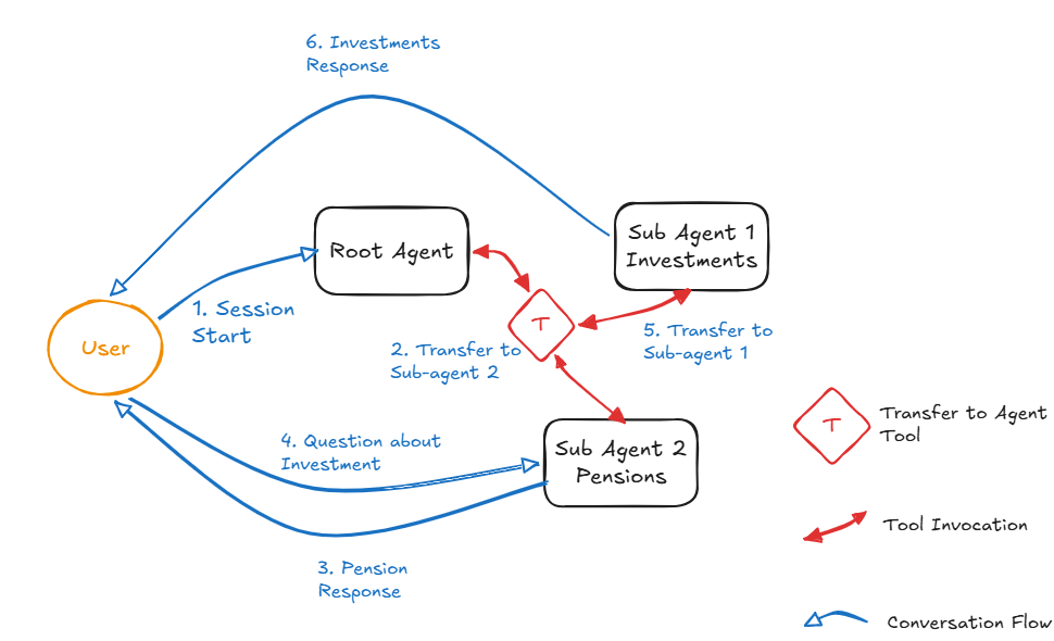
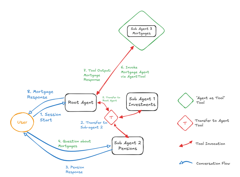
- When you attempt to replace a framework which enabled communication between agent using hidden tools (transfer_to_agent, agent_as_tool) or deterministic prebuilt workflows then it becomes more difficult to open it to provide more control and customisability.
TL;DR Verdict
Wait before switching to ADK 2.0. Don’t rush to sample the goodness of the new workflows.
Enjoy the path to production stability of ADK now that you have managed to put something in the hands of real users.
You will be ready for ADK 2.0 in 2027 or there will be much easier ways to build agents. Till then play with it, understand it.
Power users will stick with LangGraph especially with the Middleware and Deep Agents being added.
Lets Continue…
The new offerings from Google in ADK 2.0 are given below with definitions from the official website:
- Graph-based workflows: Build deterministic agent workflows with more control over how tasks are routed and executed.
- Dynamic workflows: Use code-based logic for building more complex workflows including iterative loops and complex decision-based branching.
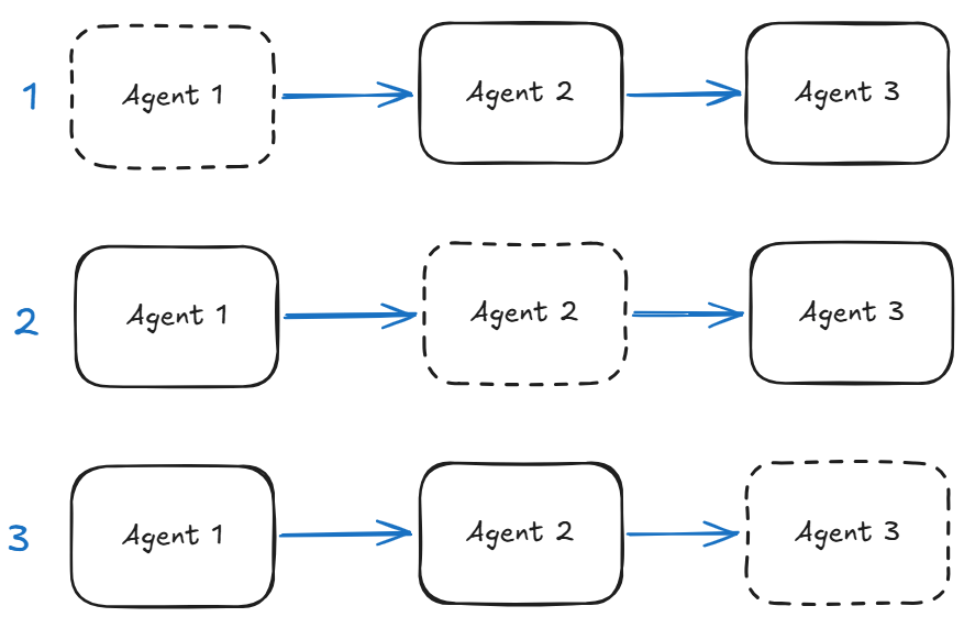
- Collaborative workflows: Build complex agent architectures with coordinator agents and multiple subagents working together.
Graph-based Workflows and General ADK 2.0
In this post we will cover the most anticipated feature in ADK 2.0 which was expected to bring it at par with LangGraph – Graph-based Workflows a.k.a. the land of commas and round brackets. We will also walk through some of the general points to note as well.
For some reason ADK 2.0 has gone for defining different types of workflows instead of just going with Nodes and Edges construct (like in LangGraph). They also use the same abstraction underneath (I guess no one has the copyright on nodes and edges) but in a complex manner.
All of the above have a few consequences:
- ADK 2.0 feels clunky and the definition of graph workflow feels like a pain.
- Input and output schemas have suddenly become super important in ADK (users of LangGraph know why) and therefore lot more thought needs to go into chaining agents, writing prompts and testing – something for ADK users to learn.
- Moving from an Agent to a Function Node when you want to use output schemas will take getting used to. The use-case is to guide LLM generation via the output schema and then feed the output into a deterministic function node for checks (the framework converts a pydantic model into a dict). If you are using a string (i.e., structureless) output then you have to take the pain to parse the LLM output which is never a trivial thing to do.
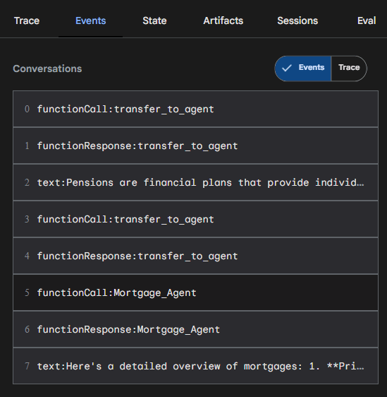
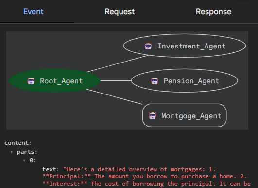
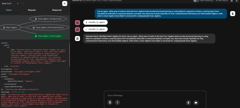
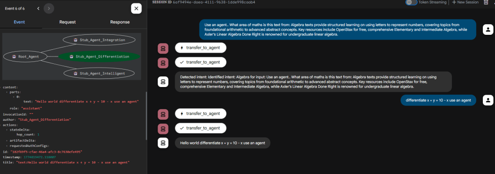
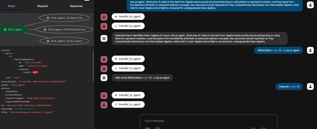
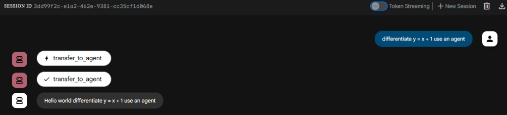
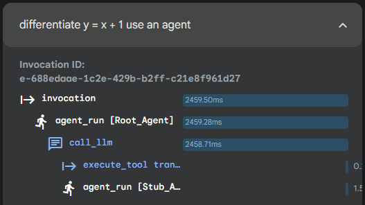
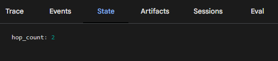
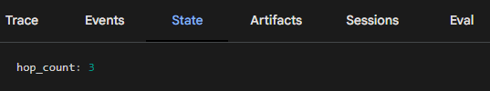
- adk web has been improved quite a bit, allowing you to see the flow through the graph and there is a .adk folder within your agent’s folder (where you have agent.py) that stores sessions data so you can debug from within VS code without having to load up adk web.
Points to Remember
Point 1
Stability – the examples work like a charm with Gemini but not so with other providers. But this is likely to improve rapidly with time.
Point 2
adk web dependency – LangChain applications do not need a dedicated runner. Easier to test and build. ADK abstraction meant you have very little to update (other than prompts or few lines of code). But with ADK2.0 will this model work when it comes to debugging chain failures – speaking from personal experience?
Point 3
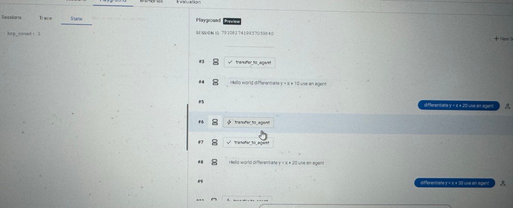
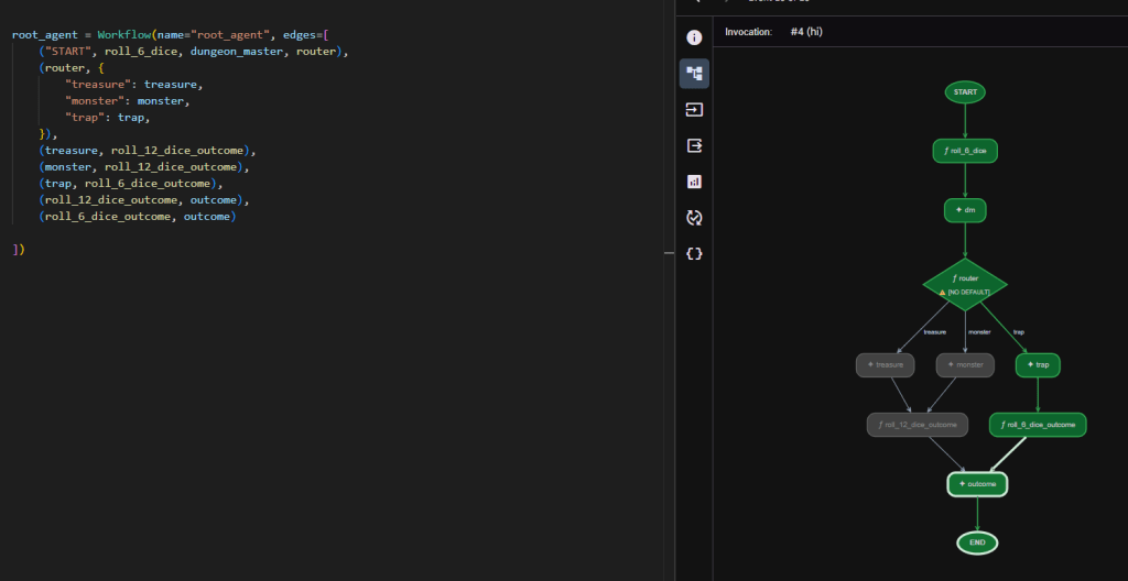
Syntax – when it comes to manually defining graphs with agents and operations I prefer the clean approach of LangGraph. ADK wins out on getting started (you do not have to worry about the graph structure). But with ADK 2.0 I find the graph representation (see example below) very difficult to read beyond the first few interconnects. All the examples on the ADK 2.0 site show graphs up to two stages which looks super easy.
A real example with a complex multi-stage graph shown below.
Point 4
Global nodes – functions or agents once declared are global entities. This means if you want to reuse the same function twice in different places within the same graph you need to re-declare it. Otherwise it will be treated as the same node and you can get weird flows and loops.
For example I have a deterministic hate_speech_check function that I want to call for checking user input and LLM output:
edges = [("START", hate_speech_check, generate, hate_speech_check)]
The above will not run and you will get a ‘unconditional cycle detected’ error.
You would have imagined the materialised graph to look like:
START -> hate_speech_check -> generate -> hate_speech_check -> END
Instead you will have to create two separate functions hate_speech_check_input() and hate_speech_check_output() that have the exact same code, and wire them up as:
edges = [("START", hate_speech_check_input, generate, hate_speech_check_output)]
Point 5
Upgrade – relatively painless, you will need to upgrade opentelemetry-sdk python package after upgrading ADK.
> pip install opentelemetry-sdk --upgrade
If you are using GCP to test your stack then you will need –allow
Misc. Points
If you see the below, don’t be confused. This ‘Agent’ is nothing but the LlmAgent aliased for easier access.
from google.adk import Agent
If you are using GCP then you will need the following additions to adk web command if you are using Cloud Shell if you want to use the local browser to access the web UI:
> adk web --allow_origins 'regex:https://.*.cloudshell.dev'
Full Code
The code for the complex graph is given below. Feel free to play around with it.
from google.adk import Workflow, Eventfrom google.adk.agents.llm_agent import LlmAgentfrom google.adk.models.lite_llm import LiteLlmfrom pydantic import BaseModelimport randomimport jsonOPENAI = "openai/gpt-4o"model = LiteLlm(OPENAI)#model = "gemini-2.5-flash"class DiceRoll(BaseModel): roll :intclass PlayerOutcome(BaseModel): outcome: strclass Result(BaseModel): player_outcome: PlayerOutcome roll: DiceRolldef roll_6_dice()->DiceRoll: return DiceRoll(roll=random.randint(1,6))def roll_12_dice_outcome(node_input:dict)->Result: outcome = Result(player_outcome=PlayerOutcome(outcome=node_input["outcome"]), roll=DiceRoll(roll=random.randint(1,6))) return outcomedef roll_6_dice_outcome(node_input:dict)->Result: outcome = Result(player_outcome=PlayerOutcome(outcome=node_input["outcome"]), roll=DiceRoll(roll=random.randint(1,6))) return outcomedef router(node_input: str): data = json.loads(node_input) print(data) return Event(route=data["result"])instruction_dungeon_master= """Roll: {DiceRoll.roll}; dice roll determines what happens to the players. Pick 'treasure' as outcome if 1,2 or a 'monster' if 3,4 or a 'trap' if 5,6. All lower case. Also return the roll. Output format: {result: outcome, roll_value: roll}"""instruction_treasure = """Generate a treasure based on strength of roll {result}. 1d12 (max value 12) will be used to determine success in the next step. Generate a safe string < 50 words."""instruction_trap = """Generate a trap based on stength of roll {result}. 1d6 (max value 6) will be used to determine success in the next step. Generate a safe string < 50 words."""instruction_monster = """Generate a monster based on strength of roll {result}. 1d12 (max value 12) will be used to determin success in the next step. Generate a safe string < 50 words."""instruction_outcome = """Generate a result based on {DiceRoll.roll} and context from previous agent."""dungeon_master = LlmAgent(name="dm",model=model, description="Greeter Agent", instruction=instruction_dungeon_master, input_schema=DiceRoll, output_key="result")treasure = LlmAgent(name="treasure", model=model, description="Treasure Generator", instruction=instruction_treasure, output_schema=PlayerOutcome )trap= LlmAgent(name="trap", model=model, description="Trap Generator", instruction=instruction_trap, output_schema=PlayerOutcome)monster = LlmAgent(name="monster", model=model, description="Monster Generator", instruction=instruction_monster, output_schema=PlayerOutcome)outcome = LlmAgent(name="outcome", model=model, description="Outcome Decider", input_schema=Result)root_agent = Workflow(name="root_agent", edges=[ ("START", roll_6_dice, dungeon_master, router), (router, { "treasure": treasure, "monster": monster, "trap": trap, }), (treasure, roll_12_dice_outcome), (monster, roll_12_dice_outcome), (trap, roll_6_dice_outcome), (roll_12_dice_outcome, outcome), (roll_6_dice_outcome, outcome) ])