Behaviours in Generative AI (Part 3)

Part 1 talks about well-behaved and mis-behaving functions with a gentle introduction using Python. We then describe how these can be used to understand the behaviour of Generative AI models.

Part 2 gets into the details of the analysis of Generative AI models by introducing a llm function. We also describe how we can flip between well-behaved and mis-behaving model behaviours.

In this part we switch to using some diagrams to tease apart our llm function to understand visually the change of behaviours.

Let us first recall the functional representation of a given LLM:

llm(instructions :str, behaviour :dict) -> output :str

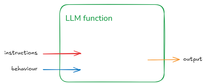
This can be shortened visualised as:

The generalisation being: for some instruction and behaviour (input) we get some output. Let us not worry about individual inputs/outputs/behaviours for the next part to keep the explanation simple. That means we won’t worry too much whether a particular output is correct or not.

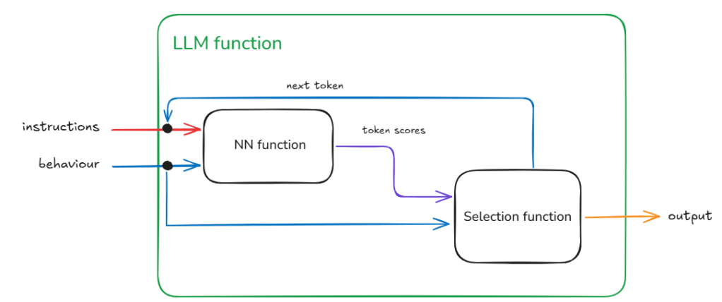
Now LLMs consist of two blocks – the ‘ye olde’ Neural Network (NN) which is the bit that is trained and the selection function. The selection function is the dynamic bit and the Neural Network the static bit. The weights that make up the NN once trained do not change.

We can represent this decomposition of the llm function into NN function and Selection function as:

The loops within llm function indicate repeated execution before some condition is met and the process ends. Another way to think about this without loops is that the calls to the NN function and the Selection function are chained – and the length of this chain unrolls through time (as determined by the past text – that includes the original instructions plus any new tokens added – and the token generated in current step).

Root Cause of the Mis-behaviour

As the name and flow in Figure 2 suggests the Selection function is selecting something from the output of the NN function.

The NN function

The output of the NN function is nothing but the vocabulary (i.e., all the tokens that the model has seen during training) mapped to a score. This score indicates the models assessment of what should be the next token (current step) based on the text generated so far (this includes the original instructions and any tokens generated in previous steps).

Now as the NN function creates a ‘scored’ set of options for the next token and not a single token that represents what goes next, we have a small problem. This is the problem of selecting from the vocabulary which token goes next.

The Selection Function

The Selection function solves this problem. This is a critical function because not only does this function influence what token is selected during the current step, it also influences the trajectory of the response one token at a time. Therefore, if a mistake is made in the early part of the generation then that is difficult to recover from. Or if a particularly important token was not selected correctly. Think for example in solving a math problem if even one digit is incorrectly selected the calculation is ruined beyond recovery. Remember, LLMs cannot overwrite tokens once generated.

The specific function we use defines the mechanism of selection. For example, we could disregard the score and pick a random token from the vocabulary. This is unlikely to give a cohesive response (output) in the end as we are basically nullifying the hard work done by the model in the current step and making it harder for it in the future steps as we are breaking any cohesive response with each random selection.

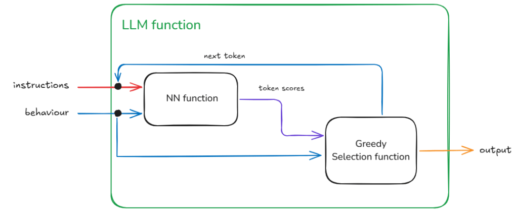
Greedy Selection

The easiest and perhaps the least risky option is to take the token with the highest score. This is least risky because given the NN function is static. Therefore, with a given instruction and behaviour we will always expect the same token scores. With greedy token selection (going for the highest score) we are going to select the same token in each step (starting from step 1). As we expect the same token scores from the start we end up building the same response again. With each step we walk down the same path as before. You will notice in Figure 3 – the overall architecture of the llm function has not changed. This is our well-behaved function – where given a specific instruction and behaviour we get the same specific output.

Sampling Selection

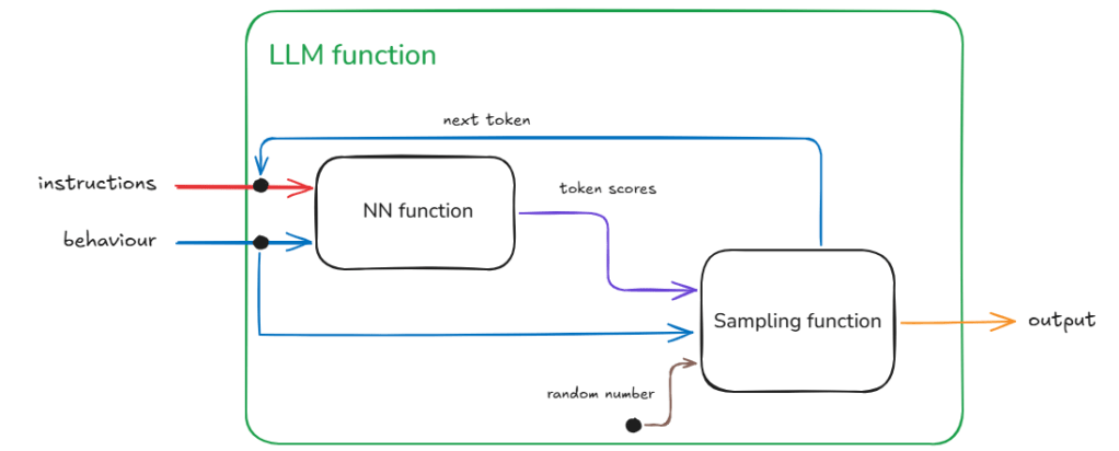
The slightly harder and riskier option is to use some kind of statistical sampling method (remember the ‘do_sample’ = True behaviour from the previous posts) which takes into account the scores. So for example, take the top 3 tokens in terms of score and select randomly from them. Or even dynamically taking top ‘n’ using some cooldown or heat-up function. The risk here is that given we are using random values there is a chance for the generation to be negatively impacted. In fact such a llm function will be badly-behaved and not compositional (see below for definition). This is so because now given the same instruction and behaviour we are no longer guaranteed to get the same output (inconsistent relation between input and output).

This inconsistency requires extra information coming from a different source given that the inputs are not changing between requests.

In Figure 4, we identify this hidden information as the random number used for sampling and the source being a random number generator. In reality we can make this random shift between outputs ‘predictable’ because we are using in actuality a pseudo-random number. With the same seed value (42 being the favourite) we will get the same sequence of random numbers therefore the same sequence of different responses for a given instruction and behaviour.

We are no longer dealing with a one-to-one relation between input and output, instead we have to think about one-to-one relationship between a given input and some collection of outputs.

I hope this has given you a brief glimpse into the complexity of testing LLMs when we enable sampling.

This inconsistency or pseudo-randomness is beneficial when we want to avoid robotic responses (‘the computer says no‘). For example, what if your family or friends greeted you in the exact same manner every time you met them and then your conversation went down the exact same arc. Wouldn’t that be boring? In fact this controlled use of randomness can help respond in situations that require different levels of consistency. For more formal/less-variable responses (e.g., writing a summary) we can tune down the randomness (using the ‘temperature’ variable – see previous post) and where we want more whimsical responses (e.g. writing poetry) we can turn it up.

Conclusion

We have decomposed our llm function into a NN and a Selection function to investigate source of inconsistent behaviours. We have discovered this is caused by hidden data in form of random variables being provided to the function for use in selecting the next token.

The concept of changing function behaviour because of extra information coming in through hidden paths is an important one.

Our brain is a big function.

A function with many hidden sources of information apart from the senses that provide input. Also because the network in our brain grows and changes as we age and learn, the hidden paths themselves must evolve and change.

This is where our programming paradigm starts to fail because while it is easy to change function behaviour it is very difficult to change its interface. Any software developer who has tried to refactor code will understand this problem.

Our brain though is able to grow and change without any major refactoring. Or maybe mental health issues are a sign of failed refactoring in our brains. I will do future posts on this concept of evolving functions.

A Short Description of Compositionality

We all have heard of the term composability – which means multiple things/objects/components together to create something new. For example we can combine simple LEGO bricks to build complex structures.

Compositionality takes this to the next level. It means that the rules for composing the components must be composable as well. That is why all LEGO compatible components have the same sized buttons and holes to connect.

To take a concrete example – language has compositionality – where the meaning of a phrase is determined by its components and syntax. This ‘and syntax’ bit is compositionality. For example we can compose the English language syntax rule of subject-verb-object to make infinitely complex sentences: “The dog barked at the cat which was chasing the rat”. The components (words) and syntax taken together provide the full meaning. If we reorder the components or change the rule composition there are no guarantees the meaning would be preserved.