The next building block for Deep Learning Networks is the Restricted Boltzmann Machine (RBM). We are going to use all that we have learnt so far in the ‘Building Blocks’ section (see here).
Bernoulli Trials
There is perhaps one small topic I should cover before we delve into the world of RBMs. This is the concept of a Bernoulli Trial (we have already hinted at it in the previous post). A Bernoulli Trial is an experiment (in the loosest sense) with the following properties:
- There are always only 2 mutually exclusive outcomes – it is a binary result
- Coin toss – can only result in a heads OR a tails for a particular toss, there is no third option
- A team playing a game with a guaranteed result, can either win OR lose the game
- The probability of both the events has a finite value (we may not know the values) which sum to 1 (because one of the two possible results must be observed after we perform the experiment)
The formulation of a Bernoulli Trial is:
P( s = 0 | 1 ) = (p^s)*(1-p)^(1- s)
If we are just interested in one of the events (say s = 1) then:
P ( s = 1 ) = p; where 0 < p < 1,
If p = 0 or 1 then it is not a probabilistic scenario – instead it becomes a deterministic scenario because we can accurately predict the result all the time (e.g.tossing a ‘fake’ Coin with two heads or two tails).
Restricted Boltzmann Machines:
A Boltzmann Machine has a set of fully connected stochastic units. A Restricted Boltzmann Machine does not have fully connected units (there are no connections between units in the same layer) but we retain the stochastic units.

When we remove the connections between units in the same layer we arrive at a now familiar structure for a feed-forward neural network. The figure above shows a simple Boltzmann Machine with 4 visible units and a RBM with 2 visible (orange) and 2 hidden units (blue).
The name Boltzmann comes from the fact that these networks learn by minimizing the Boltzmann energy of the system. In statistical physics stable systems are those that have minimum energy levels associated with the state of the different components of the system under the required constraints.
The one interesting thing that separates RBMs from normal neural networks is the stochastic nature of the units.
Taking a simple case (as done by Hinton et. al. 2006) of binary outputs (i.e. a unit is either on or off), a stochastic unit can be defined as:
“neuron-like units that make stochastic decisions about whether to be on or off”
(http://www.scholarpedia.org/article/Boltzmann_machine)
Normally (e.g. in Multi Layer Perceptrons) the activation level or score is calculated by:
- summing over the incoming scores and weights only from the previous layer (the restricted part)
- adding a bias term associated with the unit for which we are calculating the activation score
- pushing through an activation function (e.g. sigmoid or ReLU) to get an output value
The whole system is deterministic. If you know the weights, biases and inputs you can, with 100% accuracy calculate the activation scores at each layer.
To make the system stochastic with binary output (on or off), we use the sigmoid function in step 3 (as it gives values between 0 and 1) and add a fourth step to the above:
4. use the sigmoid value as the probability score for a Bernoulli Trial to decide if the unit is on or off
As a worked example:
If sigmoid (sum(x[i]w[i][j]) + bias[j]) for jth unit is = sig[j]
Then the jth unit is on if upon choosing s uniformly distributed random number between 0 and 1 we find that its value is less than sig[j]. Otherwise it is off.
So if sig[j] = 0.56 and the random number we get is 0.42 then the unit is on with an output of 1; if the random number we get is 0.63 then the unit is off with an output value of 0.
Thus higher the sigmoid output less is the chance for the unit to be turned off, however high the value there will always be a small but finite chance that the unit is off.
Similarly lower the sigmoid output higher is the chance for the unit to be turned off, however low the value there will always be a small but finite chance that the unit is on.
This leads to something very interesting:
We end up with a ‘distribution’ of outputs for every input given the weights and biases, as compared to a deterministic approach where the output is constant for a given input as long as we do not change the parameters of the model (i.e. weights and biases).
Before we move on to an example, you might be wondering why we add this extra level of complexity? How can we ever unit-test our model? Well we can easily unit-test by setting a constant seed for our pseudo-random number generator. As to why we add this extra level of complexity, the answer is simple: It allows us to give a probabilistic result which in turn allows us to deal with errors in input patterns as well as with patterns that contradict the norm (by making the network less likely to be trapped in a local minima and to not have a difficult to change association between input and output).
This is also how our brain works. If you are familiar with hash-maps or computer memory, we need the full key / address to retrieve a piece of information (i.e. it is deterministic). Even if a single character is missing or incorrect we will not be able to retrieve the required information without a lengthy search through all the keys to find the best match (which may use some sort of a probabilistic method to measure the ‘match’).
But our brain is able to retrieve the full set of information based on small samples of itself (e.g. hearing half a dialog from a movie is enough for us to recall the full scene). This is called auto-associative memory.
Worked Example:
Assume we have a RBM with 12 input units and 6 hidden units. The units are binary stochastic type.
On the input pass the 12 inputs are passed to all the 6 hidden units (through the weighted links), bias for each hidden unit is added on, sigmoid is used followed by a Bernoulli Trial to determine if the hidden unit is on or off.
Let the input also be a binary pattern. For 12 inputs there can be at most 12 bit = 4096 possible patterns. As the output at the hidden layer is also a binary pattern we know there are finite number of them (6 bits = 64 possible patterns)
Given the stochastic nature of the hidden units, for a particular binary input pattern we are likely to see some sort of a distribution across the factorial output of the hidden layer.
We can use the finite number of possible patterns to examine the distribution for a given input and see how the network is able to distinguish between patterns based on this distribution while keeping the network parameters (weights, biases) the same.
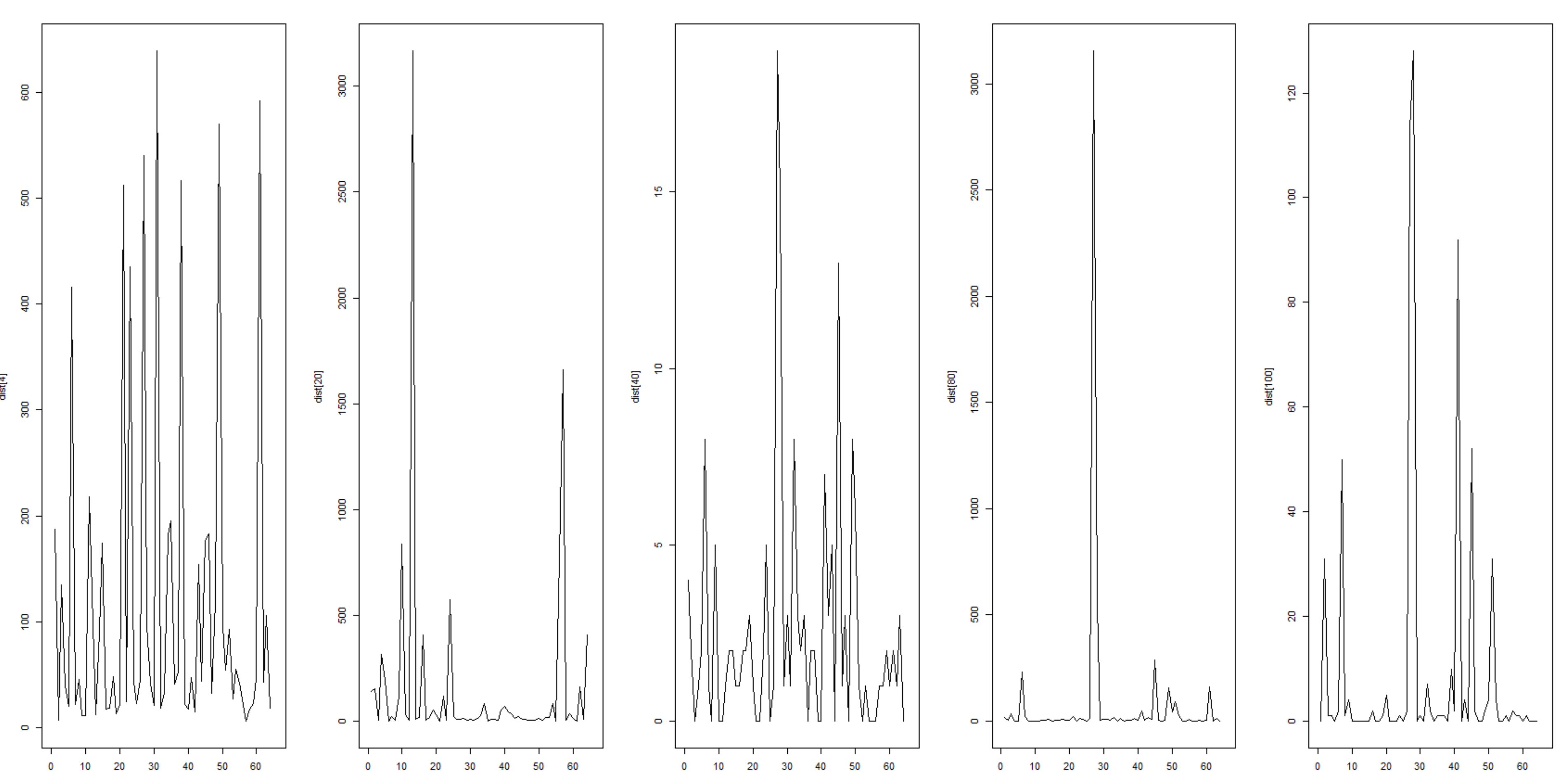
The image above shows few plots of this distribution. Each graph is created by a single 12 bit binary input pattern.
X axis are the categorical (one of 64 possible) output patterns and Y axis the count of number of times these are seen – in each graph we keep the category (X-axis) ordering the same so that we can compare the distributions across different inputs.
These are without any kind of training (i.e. weights and biases are not updated), created by pure sampling. The distributions above allow us to distinguish between different input patterns although not with a great deal of accuracy.
We can clearly see for the input vector (1 0 1 0 0 0 0 0 0 0 0 1) – 2nd graph from left, a fairly skewed distribution with high counts towards the edges, with the max being about 3165 for output (1 1 1 0 1 0); where as for the input vector (0 0 0 0 1 0 0 0 0 1 0 0) – 1st graph from left, the counts are lower and the peaks are evenly spread out.
These distributions tell us about P(h | v) for a given W and Hb which is the probability of seeing a pattern at the hidden units (h) given an input (v) for a given set of weights from visible to hidden ![]() and Hidden Unit bias values (Hb). This is also called the ‘up’ phase.
and Hidden Unit bias values (Hb). This is also called the ‘up’ phase.
We can also do the reverse of the above: P (v | h) for a given W’ and Vb which is the probability of seeing a pattern at the input units (v) given a hidden layer pattern (h) for a given set of weights from hidden to visible (W’ – transpose of W from above) and Visible Unit bias values (Vb). This is also called the ‘down’ phase.
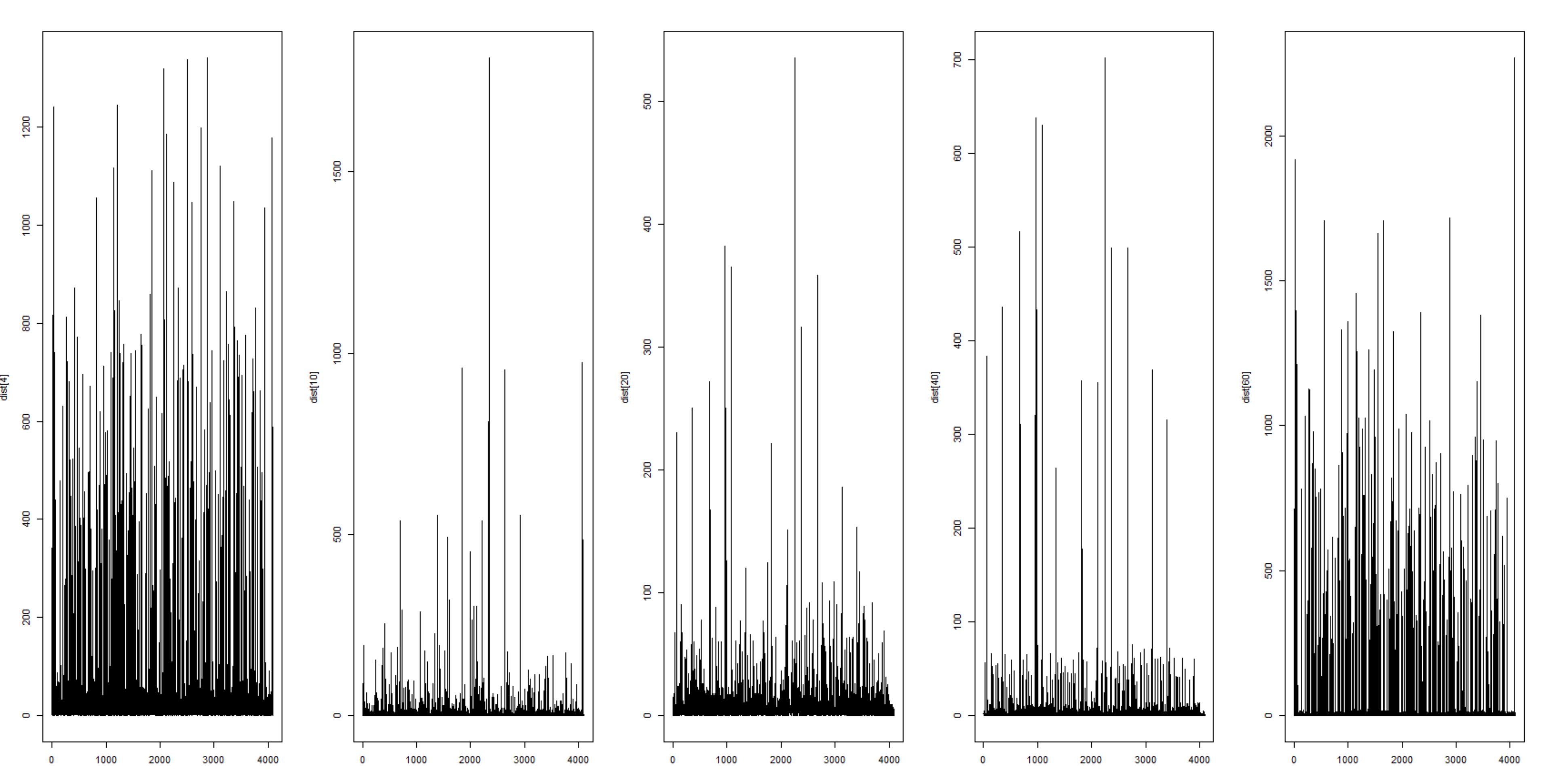
Similar to the Visible to Hidden. Here each graph represents a particular pattern at the hidden layer (one of possible 64). X axis are the 4096 possible patterns we can get at the input layer when we use the transposed Weights vector and Visible Unit bias values (along with the sigmoid – Bernoulli Trial steps). Y axis is the count.
Again we see the difference in distributions allows us to distinguish between hidden values based on the frequency of resulting input values.
Next Steps:
So far we have dealt with clear cut small dimensional inputs (e.g. 2 dimensional XOR gates, 12 bit input patterns etc.) but what if we want to process a complex picture (made up of millions of pixels in this ‘megapixel’ camera age)?
In our brain because there are no deterministic links (as a very simplistic example) it is able to associate a cartoon of a car and a picture of a car with the abstract label of ‘car’. It does high level feature abstraction to enable this probabilistic mapping. We are also able to deal with a lot of error (e.g. correctly identifying a car as drawn by a child). The one disadvantage is that we may not be able to reliably recall the same piece of information all the time (like while giving an exam we are not able to recall an answer but it comes to us some point later in time).
With a probabilistic activation it would be like the 2nd from left image in the Hidden to Visible example. Where there are clearly defined peaks for certain input patterns that result when using that hidden pattern. For example when we think of a car we get associations of ‘a cartoon car’, ‘a poster of a car’, ‘the car we drive’ etc.
If it was a deterministic system we would only ever get one input pattern for a hidden pattern (unless we updated the weights/biases). The relationship (for a generic input – whether at the ‘input layer’ or ‘hidden layer’) between inputs and outputs is always one-to-one.
Note: Don’t confuse one-to-one to mean one input to one-class. One input can activate multiple classes but the point is that it will always activate the same set of classes unless we change the weights/biases.
Also even if we updated weights and biases to take into account new training data, if the association between a feature-label pair was really strong (because of multiple examples), we would not be able to modify it easily.
That brings us to the most important piece of the puzzle – how to build a network out of such layers and then train it to distinguish between even more complex patterns.
Another key point to the training is also to make the output distributions highly distinguishable and in case of multiple peaks (i.e. multiple high probability outputs) ensure all of those are relevant. As an example for predictive text we want multiple peaks (i.e. multiple probable next words) but we want all of those to be relevant (e.g. eat should have high probability next words as ‘food’, ‘dinner’, ‘lunch’ but not ‘car’ or ‘rain’).
Contrastive Divergence allows us to do just that! We cover it next time!
As usual – please point out any mistakes… and comment if you found this useful.

2 Comments