Gibbs Sampling is a Markov Chain Monte Carlo (MCMC) method. That sounds scary but it is really not. We are going to be using an example of neural networks to understand what Gibbs Sampling is.
Sampling is just the process of extracting information about a data set (with possibly a very large number of values) using a small sub-set of it. If the sampling is done correctly we can draw a lot of interesting conclusions about the data set given the sample.
Sampling techniques are very common: e.g. by talking to a very small sub-set of the voting population after they have given their vote (i.e. an ‘exit poll’) we are able to arrive at an estimate for the voting pattern of the entire country and an approximate idea about the final result.
Many times it is not possible to take representative samples directly or through some of the other established statistical methods (like accept-reject). There are several reasons why this could be – say we cannot directly simulate the process we want to sample from or there are almost infinitely large number of possible values.
When that is the case we can use Gibbs Sampling (if certain other conditions hold).
Monte Carlo part alludes to the fact that we use ‘repeated random sampling’ from a process which is essentially a black box due to large number of interactions going on (e.g. a neural network with large number of inputs where the outputs are tied to each other via number of hidden layers with non-linear outputs).
Given a simple 2 layer network with a visible and a hidden layer – we are roughly talking about throwing in random inputs and observing what outputs we get.
The Markov Chain part alludes to the fact that we use step by step sampling with a step size of 1 – in other words a sample obtained in step T is only dependent on the sample obtained in step T-1.
When put together the process is bit like walking blindfolded around an open space, trying to figure out its shape, with the restriction that you can only move one foot at a time where as the other foot remains grounded. The more hilly sections will allow you to take only very small steps – thus you will sample more from such regions (i.e. the high probability regions), where as in the flatter areas (low probability areas) you will be able to take much bigger steps and thus generate lesser number of samples.
To mathematically define this:
Consider a bi-variate distribution p(x, y)
We are not sure how this is generated or whether p(x, y) follows any known distribution or not.
For a neural network if we say x = input at Visible Layer and y = output at Hidden Layer, then for the MNIST example reducing the input from floating point to binary (pixel on or off) gives us 2^784 possible input values. That is a staggeringly massive number of input combinations!
For all intents and purposes – the only thing we can do is repeatedly sample two conditional distributions for a finite number of values of x and y:
p(x|y) – Probability of x given y
and
p(y|x) – Probability of y given x
The above is equivalent to taking an input value and recording the output (p(y|x)) then taking an output value and reversing the direction of propagation (by transposing the weights between visible and hidden and using the visible layer bias) and recording the ‘output’ at the visible layer (p(x|y)).
Further putting conditions imposed by Gibbs Sampling and using [t] for the current step:
Starting with initial input sample x[0] (from the training data in a neural network) – we get y[0] by propagating in the forward direction and recording the output. This is equivalent to sampling from p(y|x).
This gives us the initial values for x and y = x[0], y[0].
Then we do the ‘one foot at a time’ to start Gibbs Sampling, by keeping y = y[0] (as obtained from the previous step) and propagating in the backward direction to get the next value of x = x[1]. This is equivalent to sampling from p(x|y).
The chain therefore becomes:
x[1] ~ p(x | y[0])
y[1] ~ p(y | x[1])
………………….
x[t] ~ p(x | y[t-1])
y[t] ~ p(y | x[t])
After discarding first few pairs of x,y to allow the reduction of dependence on the initial chosen value of x = x[0] we can assume that:
x[t], y[t] ~ p(x, y)
and that the sampler is now approximately sampling from the target distribution.
Once we have a sample we can effectively investigate the nature of p(x, y).
Nature of x and y:
To be very clear, x and y may appear to be scalar values but practically speaking there is no restriction. So they can be vectors or any other entity as long as we can use them as inputs to a process and record the output. For neural networks usually x is the input vector and y is the output vector. Therefore in the generic update equations:
x[t] ~ p(x | y[t-1])
y[t] ~ p(y | x[t])
x[t] is the sample of the vector x at step ‘t’ and y[t] is the sample of the vector y at step ‘t’.
y[t] ~ p(y | x[t]) is the output of the network when we supply the vector for x that we obtained in step ‘t’ as the input
Worked Example:
Assume we have a black box network with 4 bit input (giving 16 possible inputs) and 2 bit output (giving 4 possible inputs). We can designate inputs as x and outputs as y.
We cannot examine the internal structure of the network, we have no clue as to how many layers it has or what type of units make up the layers. The only thing we can do is propagate values from input to output (giving p(y | x)) and reverse propagate from output to input (giving p(x | y)). Also we assume that the network does not change as we are sampling from it.
We follow the input clamping procedure described previously and step by step take x and y samples.
Because we are looking at 16 possible inputs and 4 possible outputs we can map the sampling process (at least the first 10 steps or so) on a contour plot where we have exhaustively mapped the joint probability between x and y:
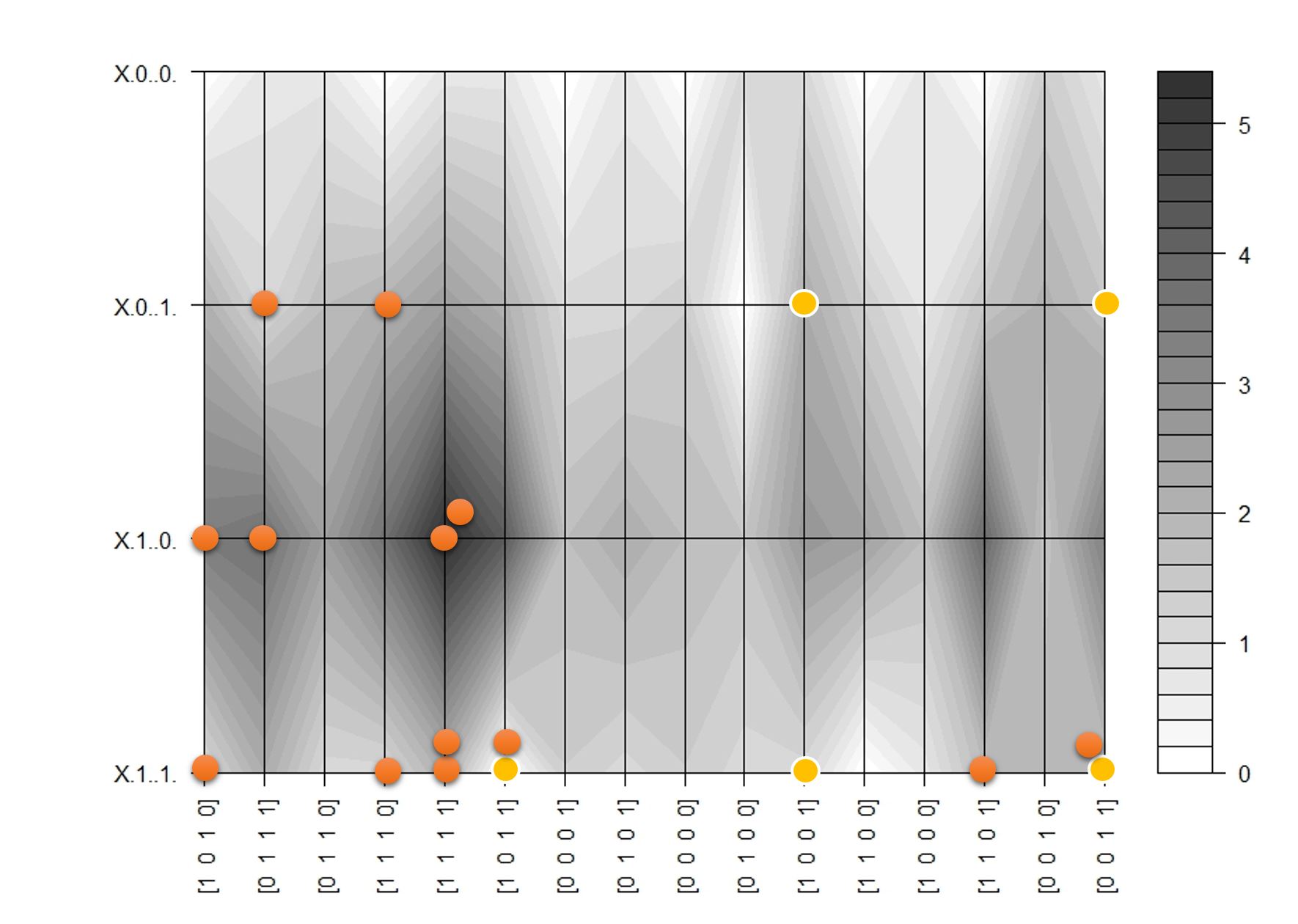
In the contour map darker regions represent areas of high probability. The dots represent sampling path with input clamped to [1, 0,1, 1]. Yellow circles show 5 initial samples as the process ‘warms up’. Subsequent samples are concentrated around the darker areas, which means we are approximately sampling from the joint distribution.
We are not always this lucky as most real world problems do not have short binary representations. We only have the black box with inputs and outputs and some training data as a very very rough guide to how the inputs are distributed, that is why we use them as the x(0) value.

1 Comment