Time-series Data in MongoDB

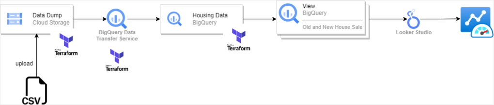
In my previous post I took the England and Wales property sale data and built a Google Cloud dashboard project using Terraform. In this post I am going to use the same dataset to try MongoDB’s new time-series capabilities.

This time I decided to use my personal server instead of on a cloud platform (e.g. using MongoDB Atlas).

Step 1: Install the latest version of MongoDB Community Server

It can be downloaded from here, I am using version 6.0.3. Installation is pretty straightforward and installers available for most platforms. Installation is well documented here.

Step 2: Create a database and time-series type of collection

Time-series collections in MongoDB are structured slightly differently as compared to the collections that store documents. This difference comes from the fact that time-series data is usually bucketed by some interval. But that difference is abstracted away by a writeable non-materialized view. In other words a shadow of the real data optimized for time-based queries [1].

The creation method for time-series collections is slightly different so be careful! In case you want to convert an existing collection to time-series variant then you will have to dump the data out and create a time-series collection into which you import the dumped data. Not trivial if you are dealing with large amounts of data!

There are multiple ways of interacting with MongoDB:

  • Mongo CLI client
  • Your favourite programming language
  • MongoDB Compass GUI client

Let us see how to create a time-series collection using the CLI and Python:

CLI:

db.createCollection(
"<time-series-collection-name>", 
{
    timeseries : 
    {
          timeField:"<timestamp field>", 
          metaField: "<metadata group>", 
          granularity:"<one of seconds, minutes or hours>"
    }
})

Python:

db.create_collection(
    "<time-series-collection-name>",
    timeseries = {
        "timeField": "<timestamp field>",
        "metaField": "<metadata group>",
        "granularity": "<one of seconds, minutes or hours>"
     })

The value given to the timeField is the key in the data that will be used as the basis for time-series functions (e.g. Moving Average). This is a required key-value pair.

The value given to the metaField is the key that represents a single or group of metadata items. Metadata items are keys you want to create secondary indexes on because they show up in the ‘where’ clause. This is an optional key-value pair.

The value for granularity is set to the closest possible arrival interval scale for the data and it helps in optimizing the storage of data. This is an optional key-value pair.

Any other top level fields in the document (alongside the required timeField and optional metaField) should be related to the measurements that we want to operate over. Generally these will be the values that we use an aggregate function (e.g. sum, average, count) over a time window based on the timeField.

Step 3: Load some Time-series Data

Now that everything is set – we load some time series data into our newly created collection.

We can use mongoimport CLI utility, write a program or use MongoDB Compass (UI). Given this example is with the approx 5gb csv property sale data I suggest using either mongoimport CLI utility or MongoDB Compass. If you want to get into the depths of high performance data loading then the ‘write a program’ option is quite interesting. You will be limited by the MongoDB driver support in the language of choice.

Adding the command I used:

mongoimport –uri=mongodb://<mongodb IP>:27017/<database name>

–collection=<collection_name> –file=<JSON file path> –jsonArray

The mongoimport CLI utility takes approximately 20 minutes to upload the full 5gb file when running locally. But we need to either convert the file from csv into json (fairly easy one time task to write the converter) or to use a field file as the original csv file does not have a header line.

Note: You will need to convert to JSON if you want to load into a time-series collection as CSV is a flat format and time-series collection requires a ‘metaField’ key which in this case points to a nested document.

Compass took about 1 hour to upload the same file remotely (over the LAN).

Compass is also quite good to test the data load. If you open up the collection in it you will see the ‘Time-Series’ badge next to the collection name (‘price_paid’ in the image below).

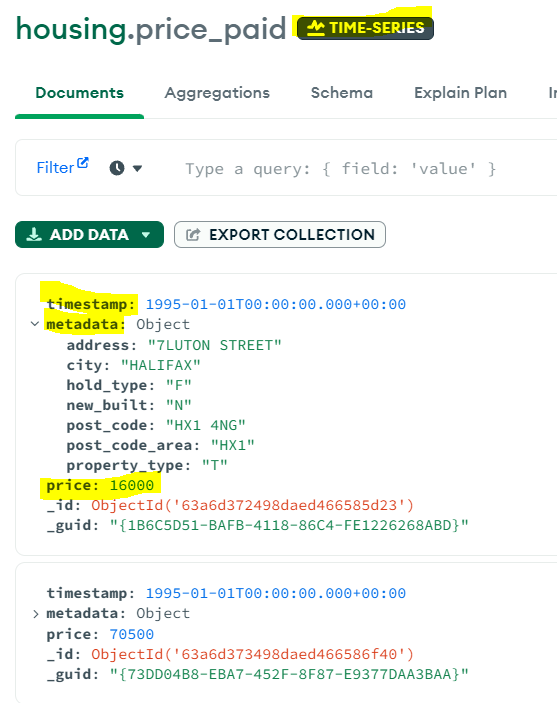
Let us see example of a single document (image above) to understand how we have used the timeField, metaField and top level fields.

timeField: “timestamp” – the date of the transaction

metaField: “metadata” – address, city, hold-type, new-built, post_code and area, property type – all the terms we may want to query by

top level: “price” – to find average, max, min etc. of the price range.

Step 4: Run a Query

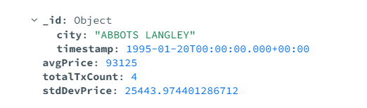
Now comes the fun bit. I give an example below of a simple group-by aggregation that uses the date of transaction and the city that the property is in as the grouping clause. We get the average price of transactions, the total number of transactions and standard deviation of the price in that group:

{
  _id: {
    city: "$metadata.city",
    timestamp: "$timestamp",
  },
  avgPrice: {
    $avg: "$price",
  },
  totalTxCount: {
    $sum: 1,
  },
  stdDevPrice: {
    $stdDevSamp: "$price",
  },
}

Sample output of the above (with 4,742,598 items returned):

Step 5: Run a Time-series Query

We are close to finishing our time-series quest! We have data grouped by city and transaction date now we are going to calculate the Moving Average.

{
    partitionBy: "$_id.city",
    sortBy: {
         "_id.timestamp": 1,
    },
    output: {
         "window.rollingPrice": {
             $avg: "$avgPrice",
             window: {
                  range: [-6, 0],
                  unit: "month",
             },
          },
    },
}

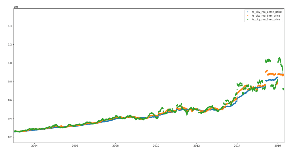
The above aggregation query uses the ‘setWindowFields‘ stage – partitioning by ‘city’ and sorting by the time field (‘timestamp’). We use a window of 6 months before the current timestamp value to calculate the 6 month moving average price. This can be persisted to a new collection using the ‘out‘ stage.

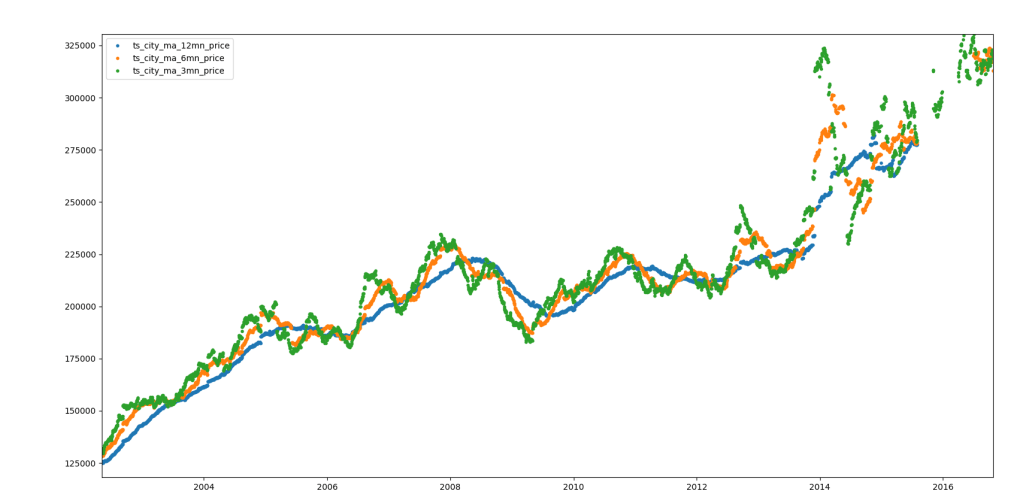
The image above shows the 3 (green), 6 (orange) and 12 (blue) month moving average price for the city of Bristol. The image below shows the same for London. These were generated using matplotlib via a simple python program to query the relevant persisted moving average collections.

Reflecting on the Output

I am using an Intel NUC (dedicated to MongoDB) with an i5 processor and 24GB of DDR4 RAM. In-spite of the fact that MongoDB attempts to corner 50% of total RAM and the large amount of data we have, I found that 24GB RAM is more than enough. I got decent performance for the first level grouping queries that were looking at the full data-set. No query took more than 2-3 minutes.

When I tried the same query on my laptop (i7, 16GB RAM) the execution times were far longer (almost double).

Thank you for reading this post!

Housing Data on GCP using Terraform

The UK Government provides data for property transactions for all sales in England and Wales. This data is updated monthly and all the files can be found: https://www.gov.uk/government/statistical-data-sets/price-paid-data-downloads

The single CSV datafile (going back almost 30 years) is approximately 5gb.

I wanted to use this as a target to learn more about the cloud as it is not a ‘toy’ dataset. The idea is to do everything using cloud components and services. I decided to use GCP as it has a generous ‘free’ tier.

Also I wanted to automate as much of the deployment as I could using Terraform Infrastructure as Code (IaC). This makes maintaining the project a lot easier as well as making changes. One of the things to remember is that even with IaC there are many components that support ‘config change’ by tearing down and creating the resource again.

Terraform IaC

Terraform is at its core four things:

  1. A Language (HashiCorp Configuration Language) to describe configuration to be applied
  2. A Set of Providers that convert configuration described in the Terraform language to API commands for the target platform
  3. The ‘terraform’ command that brings together the Terraform config files and Providers
  4. Configuration state store

The first feature allows one language to describe all kinds of configurations (IaC). The second feature abstracts away the application of that config via Providers (adapters). The third feature allows us to interact with Terraform to get the magic to work. The fourth feature provides a ‘deployed’ state view.

A key artefact when applying config is what Terraform calls a ‘plan’ that explains what changes will be made.

Terraform interacts with target providers (like Google Cloud, AWS, Azure) using ‘provider’ code blocks and with components made available by those providers using ‘resource‘ code block. Each ‘resource’ block starts off with the resource-type it represents and its name.

One thing to remember is that a Provider (defined using the ‘provider’ code block) has no special way of interacting with the target provider. It is ultimately dependent on the APIs exposed by the target provider. If a provider forces you to use their UI for certain management scenarios then you won’t be able to use Terraform.

Also providers generally have their own IaC capabilities. For example the Google Cloud Deployment Manager and the AWS CloudFormation.

The Project (ver. 1)

Given that I am using the ‘free’ tier of Google Cloud and want to learn those capabilities step-by-step (while avoiding the ‘paid’ tier) I am building my cloud architecture using basic services such as Google Cloud Storage, BigQuery and Looker.

My cloud architecture v1 looks like this:

The CSV file containing the full housing data set gets uploaded to GCS bucket. From there a BigQuery Data Transfer Service parses the CSV file and injects it into a BigQuery table. We then run a set of saved queries to create views for our dashboard. Finally those views are consumed from a Looker Studio Dashboard.

The Terraform symbol in the figure indicates automated resource creation. In the current version I am auto-creating the GCS bucket, BigQuery Data Transfer Service and the BigQuery table. The CSV upload can also be automated by using the ‘google_storage_bucket_object’ resource.

The reason I started off with the above pieces of automation is because I found taking these steps again and again to be very frustrating – especially creating the Table in BigQuery as the schema is fairly complex as well as creating a data transfer job with correct parsing parameters.

The Implementation

The resulting dashboard can be seen here: https://datastudio.google.com/reporting/138a9b59-7cf6-4b04-9c19-fb744b1c7854

You can filter by property type: Terraced (T), Flat (F), Other (O), Semi-detached (S) and Detached (D). Then you can see how the combined old + new transactions signal splits if we see only the New Builds (top – right) or only the Resales (Old Builds in bottom – right).

The Terraform code is given below, items in <> need to filled in before running the script:

#using existing project - otherwise we can create a new project as well
provider "google" {
    project = "<your project name>"
}
#setup bigquery dataset
resource "google_bigquery_dataset" "housing2" {
    dataset_id = "housing_dump_2"
    location = "us"
    delete_contents_on_destroy = true
    labels = {
      env = "default"
    }
}
#setup gcs bucket
resource "google_storage_bucket" "housing_bucket" {
  name = "<your bucket name>"
  location = "US-east1"
  force_destroy = true
  public_access_prevention = "enforced"
  uniform_bucket_level_access = true
  storage_class = "STANDARD"


}
# setup bigquery data transfer 
# to parse CSV file in gcs bucket into bigquery table
resource "google_bigquery_data_transfer_config" "default" {
  
  display_name = "mirror_data_dump"
 
  destination_dataset_id = google_bigquery_dataset.housing2.dataset_id
  data_source_id = "google_cloud_storage"
  params = {
    destination_table_name_template = "housing_data"
    write_disposition = "MIRROR"
    data_path_template = "gs://<gcs bucket>/<csv file name>"
    file_format="CSV"
    field_delimiter=","
    quote = "\""
    delete_source_files = "false"
    skip_leading_rows = "0"
  }
  schedule_options  {
      disable_auto_scheduling = true
  }
     
}
#create bigquery table with the correct schema to support data transfer
resource "google_bigquery_table" "default" {
    dataset_id = google_bigquery_dataset.housing2.dataset_id
    table_id = "housing_data"
    deletion_protection = false
    time_partitioning {
      type = "DAY"
    }
    labels = {
      env = "default"
    }
    schema = <<EOF
    [
  {
    "name": "transaction_guid",
    "mode": "NULLABLE",
    "type": "STRING",
    "description": "Transaction GUID",
    "fields": []
  },
  {
    "name": "price",
    "mode": "NULLABLE",
    "type": "INTEGER",
    "description": "Price",
    "fields": []
  },
  {
    "name": "date_transfer",
    "mode": "NULLABLE",
    "type": "TIMESTAMP",
    "description": "Date of Transfer",
    "fields": []
  },
  {
    "name": "postcode",
    "mode": "NULLABLE",
    "type": "STRING",
    "description": "Postcode",
    "fields": []
  },
  {
    "name": "property_type",
    "mode": "NULLABLE",
    "type": "STRING",
    "description": "D = Detached, S = Semi-Detached, T = Terraced, F = Flats/Maisonettes, O = Other",
    "fields": []
  },
  {
    "name": "old_new",
    "mode": "NULLABLE",
    "type": "STRING",
    "description": "Old or New build",
    "fields": []
  },
  {
    "name": "duration",
    "mode": "NULLABLE",
    "type": "STRING",
    "description": "\tRelates to the tenure: F = Freehold, L= Leasehold etc.",
    "fields": []
  },
  {
    "name": "PAON",
    "mode": "NULLABLE",
    "type": "STRING",
    "fields": []
  },
  {
    "name": "SAON",
    "mode": "NULLABLE",
    "type": "STRING",
    "fields": []
  },
  {
    "name": "Street",
    "mode": "NULLABLE",
    "type": "STRING",
    "fields": []
  },
  {
    "name": "Locality",
    "mode": "NULLABLE",
    "type": "STRING",
    "fields": []
  },
  {
    "name": "City",
    "mode": "NULLABLE",
    "type": "STRING",
    "fields": []
  },
  {
    "name": "District",
    "mode": "NULLABLE",
    "type": "STRING",
    "fields": []
  },
  {
    "name": "county",
    "mode": "NULLABLE",
    "type": "STRING",
    "fields": []
  },
  {
    "name": "ppd_category",
    "mode": "NULLABLE",
    "type": "STRING",
    "description": "A = Standard Price Paid entry, includes single residential property sold for value.\nB = Additional Price Paid entry including transfers under a power of sale/repossessions, buy-to-lets",
    "fields": []
  },
  {
    "name": "record_status",
    "mode": "NULLABLE",
    "type": "STRING",
    "fields": []
  }
]
EOF
}

To run the above simply save it as a Terraform file (extension .tf) in its own folder. Make sure Terraform is installed, in the path and associated with your GCP account. Then run from the same directory as the .tf file:

terraform validate to validate the file

terraform plan to review the config change plan without deploying anything

terraform apply to apply config changes to selected Google Cloud project

terraform destroy to destroy changes made by apply