Talking with your Data (SQL)

This post is about testing text-to-SQL generation capabilities with human in the loop. The broader use-case is around being able to talk with your data for generating insights.

The results will blow your mind!

So instead of creating dashboards around questions (e.g., which product had the highest sales in the previous 3 months?) you could ask any question and an automated system would go and query the right data to return a response in a human understandable way.

Model: For this post I am using the Defog text-to-SQL model (8 billion parameters) based on Llama-3 from Hugging Face: defog/llama-3-sqlcoder-8b. This is a relatively new model (mid-May 2024).

Infrastructure: the model is running locally and takes about 30gigs of RAM for the prompts I used. I use a SQLite 3 database as a backend.

Model Deployment: I have created a python flask web-server (read more here) that allows me to deploy any model once when the server starts and then access it via a web-endpoint.

Software: A python web-client for my model server that takes care of prompting, workflow, human-in-the-loop, and the integration with other components.

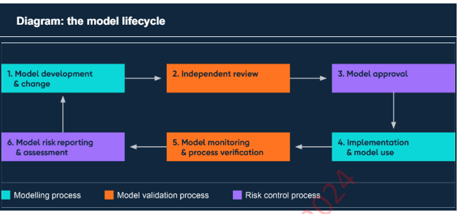
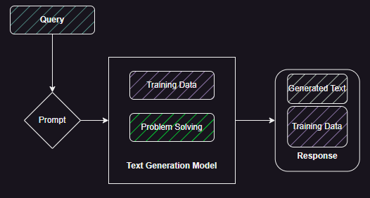
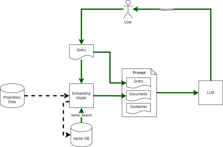
Figure 1 shows the flow of the main app and its interactions with the LLM and the SQL database.

Figure 1: Flow of the application (green arrow) and interactions with the LLM and Database.

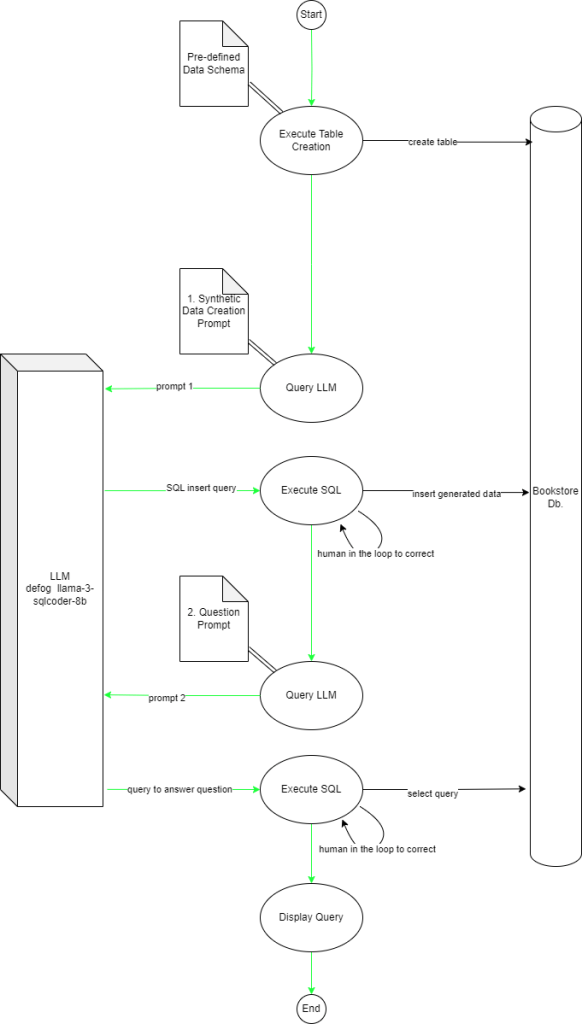
Challenges to overcome: This is a complex use-case that covers synthetic data creation based on schema, Insert, and Select use-cases against a multi-table database. This requires the LLM to:

  1. Understand the Data Definition (in SQL)
  2. Correctly generate synthetic data based on the definition
  3. Correctly generate the insert statements (in the correct order as the foreign keys have a not null clause)
  4. Understand the user’s question
  5. Convert the question into a valid SQL query with joins and other operations as required

Keep in mind that this is not a gazillion parameter GPT-4o or Gemini. This is not even the larger variant of the sqlcoder model with 34 billion parameters. This is the humble 8b parameter version!

The Schema: The schema simulates a book store with four tables – authors, books, inventory, and transactions. The relationships are as follows:

  1. Author (1) -> (*) Books
  2. Books (1) -> (1) Inventory
  3. Books (1) -> (1) Transactions

Synthetic data is generated for all the tables based on directions given in the first Prompt (prompt 1).

The question (Which Author wrote the most books?) requires a join between the Author and Books tables.

The Stages

Posting some snippets of the output here, the full code can be found on my Github repo.

Creating the Tables

A simple data definition (DDL) script that is run by the python client.

create table authors (author_id varchar(20) primary key not null, name text not null);

create table books (book_id varchar(20) primary key not null, name text not null, author_id varchar(20) not null, FOREIGN KEY(author_id) REFERENCES authors(author_id));

create table inventory (inv_id varchar(20) primary key not null, book_id varchar(20) not null, quantity int not null, FOREIGN KEY(book_id) REFERENCES books(book_id));

create table transactions(tx_id varchar(20) primary key not null, book_id varchar(20) not null, quantity_sold int not null, sale_date date not null, FOREIGN KEY(book_id) REFERENCES books(book_id));

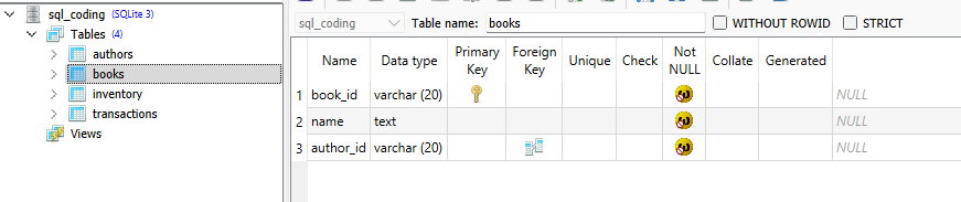
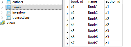
We can see the output above with the full structure of the books table. I am using SQLite Studio to view the structure and data only, all changes are made programmatically. This is still using python sqlite libraries so nothing magical yet.

Creating and Inserting Synthetic Data

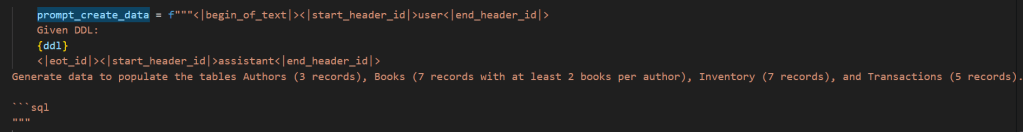
For the next step (creating and inserting synthetic data) we bring in the LLM (sqlcoder). The prompt used can be seen in Figure 2. The ddl placeholder just injects the above create SQL statements to provide information about the structure of tables and relationships between them. We also define the number of records per table and some other constratins.

Figure 2: Prompt for generating synthetic data.

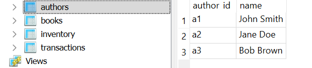
The LLM returns the following response to the above prompt. We can see the constraints for number of records and number of books per author are respected.

INSERT INTO authors (author_id, name) VALUES ('a1', 'John Smith'), ('a2', 'Jane Doe'), ('a3', 'Bob Brown');

INSERT INTO books (book_id, name, author_id) VALUES ('b1', 'Book1', 'a1'), ('b2', 'Book2', 'a1'), ('b3', 'Book3', 'a2'), ('b4', 'Book4', 'a2'), ('b5', 'Book5', 'a3'), ('b6', 'Book6', 'a3'), ('b7', 'Book7', 'a1');

INSERT INTO inventory (inv_id, book_id, quantity) VALUES ('i1', 'b1', 5), ('i2', 'b2', 3), ('i3', 'b3', 4), ('i4', 'b4', 2), ('i5', 'b5', 6), ('i6', 'b6', 8), ('i7', 'b7', 9);

INSERT INTO transactions (tx_id, book_id, quantity_sold, sale_date) VALUES ('t1', 'b1', 2, '2022-01-01'), ('t2', 'b2', 1, '2022-01-02'), ('t3', 'b3', 3, '2022-01-03'), ('t4', 'b4', 4, '2022-01-04'), ('t5', 'b5', 5, '2022-01-05');

Below we can see a screenshot from SQLiteStudio after the generated insert statements were run. We can see the SQL generator has clearly picked out the schema of each table and the relationships between them just from the data

The stage is now set for us to move to ‘talking to your data’.

Asking A Few Questions

The first question we ask is: Tell me which author has written the most books?

If you are familiar with the Spider 1.0 challenge from Yale (for Text-to-SQL) this above question is a medium complexity one because the model has to correctly identify the need for a join and populate the current table and field names given the schema.

The prompt template is given below. The placeholder question1 is what we use for questions. In this case I created two separate prompts but the structure is exactly the same and we can easily convert it into a function that takes in a question as a string and outputs the filled template.

Figure 3: Prompt template for a question.

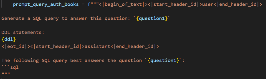
The entry below shows the SQL query generated by the model and the Query Output when that query is executed.

SQL Query:
WITH BookCounts AS (SELECT a.name, COUNT(b.book_id) AS book_count FROM authors a JOIN books b ON a.author_id = b.author_id GROUP BY a.name) SELECT name, book_count FROM BookCounts ORDER BY book_count DESC LIMIT 1;

Query Output: ('John Smith', 3)

The Query output gives the correct answer.

The next question is: Tell me which books had the highest sales?

Now the key point about this query is that I am not talking about the book that sold the most, instead I am talking about the ‘books’. The model recognises this. We use the same template as above but just replace the text in the question1 placeholder with the above question.

SQL Query:
WITH TotalSales AS (SELECT b.book_id, SUM(t.quantity_sold) AS total_sales FROM transactions t JOIN books b ON t.book_id = b.book_id GROUP BY b.book_id) SELECT bs.book_id, bs.total_sales FROM TotalSales bs ORDER BY bs.total_sales DESC NULLS LAST LIMIT 5;

Query Output:
('b5', 6)
('b4', 4)
('b2', 3)
('b1', 2)
('b3', 1)

The Query output once again gives the correct output. The model has interpreted the need to give the top n results. In fact the model has gone a step further and set n to ‘5’, so it returns the top 5 books in terms of sales using a join between the transaction and books table.

The final question is: Tell me which author has the most sales?

Looking at Spider 1.0 this would come in the Hard category.

This time I wanted to check a question that requires more than one join and a group operation. So in this case you need to join the transactions and books table and then group and join the result to the authors table to cater for the fact that a single author may have written multiple books.

SQL Query:
WITH TotalSales AS (SELECT b.author_id, SUM(t.quantity_sold) AS total_quantity_sold FROM transactions t JOIN books b ON t.book_id = b.book_id GROUP BY b.author_id), RankedAuthors AS (SELECT a.author_id, a.name, ts.total_quantity_sold, RANK() OVER (ORDER BY ts.total_quantity_sold DESC) AS sales_rank FROM authors a JOIN TotalSales ts ON a.author_id = ts.author_id) SELECT ra.name, ra.total_quantity_sold FROM RankedAuthors ra WHERE ra.sales_rank = 1;

Query Output:
('Jane Doe', 6)

Once again the result is correct! Amazing stuff as promised! I have tried this demo more than 20 times and it worked flawlessly.

The code for the SQL LLM Server https://github.com/amachwe/gen_ai_web_server/blob/main/sql_coding_server.py

The code for the SQL LLM Server client: https://github.com/amachwe/gen_ai_web_server/blob/main/sql_coding_client.py

Have fun!

Web-server for LLMs

One thing that really bugs me when running larger LLMs locally is the load time for each model. Larger the on-disk size of the model, the longer it takes for the model to be ready to query.

One solution is to run the model in a Jupyter notebook so we load it once and then query as many times as we want in subsequent code blocks. But this is not ideal because we can still have issues that require us to restart the notebook. These issues usually have little to do with the Gen AI model itself (which in most use-cases is treated as a closed box).

Another requirement is to be able to run your application and your LLM on different machines/instances. This can be a common requirement if you want to create a scalable Gen-AI based app. This is the main reason we have services like the Google Model Garden that don’t require you to ‘host’ models and provide API-based access instead.

To get around this I developed a web-server using python flask that can load any model accessible through the huggingface transformers library (using a plugin approach). This is mainly useful for testing and learning but can be made production ready with little effort.

The code can be found here: https://github.com/amachwe/gen_ai_web_server

Key steps to wrap and setup your model web-server:

  1. Load the tokenizer and model using the correct class from the huggingface transformers python library.
  2. Create the wrapped model using selected LLM_Server_Wrapper and pass that to the server.
  3. Start the server.

The above steps shown as code below. Also available in the llm_server.py file in the linked GitHub repo above.

Will share further examples of how I have been using this…

… as promised I have now added a client to help you get started (see link below).

Simple Client

This client shows the power of abstracting the LLM away from its use. We can use the “/info” path to get the prompting hints from the wrapped model. This will help the client create the prompt properly. This is required because each model could have its own prompting style.

Indian General Elections (2024)

Numbers are really beautiful and can often illuminate hidden corners of a complex situation. But before we start, I want to congratulate the citizens of India on an amazing election during record breaking heatwaves.

The results was a transition from Modi 2.0 to NDA 3.0 (previous two being under Mr Vajpayee) with BJP emerging as the single largest party but falling short of an absolute majority by about 32 seats.

In many ways this is a good situation that BJP is on relatively solid ground to be able to support the coalition with clear dependency on its other members to encourage more consultative approach to governance.

Figure 1: Comparing Total Parliamentary Seats in a state vs % of Seats won by NDA. Yellow line shows the half way mark (50% seats).

Back to the numbers…

I only want to show one graph to help explain why we have the given situation. Figure 1 above shows total seats in a State against the win % (in terms of number of seats won by the BJP).

To get absolute majority the states below the orange line had to be much closer to it or in case of Uttar Pradesh, above it.

What didn’t help was the fact that states in the centre and right (those with larger number of seats in the Parliament) ended up below the yellow line (50% seat win line).

The states below or on the yellow line but above the orange line needed to be above the yellow line. For example, this time BJP lost one seat in Jammu and Kashmir – which took the win % below the 50% line (2 out of 5 seats) but still kept it above the orange line (lower envelope).

I want to add one more piece of information to the graph. The trend in voter turnout. In Figure 2 (below) we see that the red marked states (voter turnout was lower than in 2019) are mostly above the 50% win rate (yellow) line. Those below the orange line are mostly green (voter turnout higher than 2019).

Figure 2: Same plot with colour coded states based on voter turnout trend (green for increase, red for decrease, and black for no data).

My first hypothesis is that BJP voters were far more resilient and enthusiastic about voting.

My second hypothesis is that those supporting non-BJP candidates were not convinced about their chances in front of the shock and awe campaign undertaken by the BJP.

New Regulation for AI, Prudential Regulation Authority: Supervisory Statement 123

Effective from 17th May 2024.

The PRA Supervisory Statement 123

Model risk management (MRM) is a process the regulator expects all UK banks to implement if they are using any kind of model-based decision making. This is not a ‘new’ process for the development, verification, monitoring, and reporting of machine learning, statistical, and rule-based decision models. The end-to-end process is shown in the image below. There are additional components like the Model Inventory.

Why is this important?

This is important because MRM covers any type of AI model, doesn’t matter if you build it or you buy it. Doesn’t matter if it is a small XGBoost model or a Large-Language Model. There are clear guidelines for what is expected as part of the modelling process, validation process, and the risk control process.

I don’t think anyone knows how this applies to LLMs. If anyone has ideas I am happy to learn more.

Especially, third-party LLMs like Llama, Mistral, etc. where details of the modelling process are hidden behind intellectual property protection. Model validation and risk management are also new things when it comes to Large-Language Models. The main reason being that we cannot easily tie these to a specific use-case. All you need to do to change the behaviour of a LLM is to change the prompt. You can make it summarise text and then change the prompt to make it answer a question.

The Context

Let us look at various important definitions and concepts presented in SS 123.

Who is covered by SS 123

All regulated UK banks and building societies.

Why do we need SS 123

To manage Model Risk – this is the risk to the consumer, the bank, and/or the wider economy arising from the inappropriate use of models or due to errors made by the models.

What is covered by SS 123

Business decision making, risk management, and reporting – wide coverage.

What is a Model?

SS 123 defines a model (Principle 1.1 [a]) on pages 8 and 9 as:

A model is a quantitative method, system, or approach that applies statistical,
economic, financial, or mathematical theories, techniques, and assumptions to
process input data into output. The definition of a model includes input data that are
quantitative and / or qualitative in nature or expert judgement-based, and output that
are quantitative or qualitative.

Why do I think this covers LLMs? Because Principle 1.1 [a] explicitly mentions qualitative inputs and outputs, including expert judgement-based. Expert judgement-based aligns nicely with a ‘prompt’ for the LLM.

Additionally SS 123 Principle 1.3 talks about risk-based model tiering in order to identify and classify models that represent the highest risks as it goes through the model lifecycle. Why do I think LLMs should be in the ‘highest’ risk (i.e., most effort)? Let us understand through the ‘materiality’ (impact) and ‘complexity’ rating as described in SS 123.

Materiality

Size-based measures based on exposure, number of customers, and market values and qualitative factors related to its importance to informing business decisions.

LLMs are expected to be used by a large number of related use-cases. These could be as a shared instance or multiple instances of the same model. Therefore, the exposure could be widespread. Furthermore the use of LLMs in summarising, Q&A, and augmentation are all examples of ‘informing’ business decisions. For example, an agent using Gen AI-based Q&A system could rely on interpretation and summarisation provided by a Gen AI model.

Complexity

Various factors including: nature and quality of input data, choice of methodology, requirements and integrity of implementation, and the extensiveness of use of the model. But that is not all, when it comes to ‘newly advanced approaches or technologies’ (page 10), the complexity assessment may also consider risk factors related to: use of alternative and unstructured data, and measures of a model’s interpretability, explainability, transparency, and the potentials for designer or data bias to be present.

This last bit is written for LLMs: the use of unstructured data like text, images, and video. Evaluation of model interpretability, explainability, bias etc. are all important unsolved issues with LLMs.

Finally there is requirement for independent assessment and reassessment of models. How would this work for LLMs? Who would do the assessment?

Work To Do Ahead!

Lot of work still needs to be done clearly by all banks and regulated entities but there are many critical unknowns in this area. Key unknowns are how do we carry out independent reviews without clear guidelines? How do we verify the model build and ongoing testing of LLMs, especially those built by third-parties.

Within a bank a key role will be that of the model owner as they will be accountable for model use and with third-party LLMs will not be able to control the development of the same. Does this mean the end-state for LLMs is all about self-build, self-manage, and self-govern? Because there are two other roles: model users and model developers and the risk starts to build up right from when we start planning the model (e.g., selecting datasets and the LLM task).

Finally, the proportionality of MRM principles implies the largest entities (banks) need to make the most effort in this. In fact even simple requirements like tracking models in a model inventory (Principle 1.2) – the type of information you would need to track for LLMs is not straightforward as compared to a traditional machine learning model.

Saving and Using Model Artefacts

One of the keys requirements for creating apps that use AI/ML is the ability to save models after training, in a format that can be used to share and deploy the model.

This is similar to software packages that can be shared and used through language specific package managers such as Maven for Java.

When it comes to models though there multiple data points that need to be ‘saved’. These are:

1) the model architecture – provides the frame to fit the weights and biases in as well as any layer specific logic and custom layer definitions.

2) the weights and biases – the output of the training process

3) model configuration elements

4) post processing (e.g., beam search)

We need to ensure that the above items as they exist in memory (after training) can be serialised (“saved to disk”) in a safe and consistent way that allows it to be loaded and reused in a different environment.

All the major ML libraries in python provide a mechanism to save and load models. There are also packages that can take a model object created by these libraries and persist them on disk.

TLDR: Jump straight to the Conclusions here.

Major Formats for Saving the Model

The simplest type of model is one that has an architecture with no custom layers or complex post processing logic. Basically, it is just a tensor (numbers arranged in a multi-dimensional array). Some examples include: linear regression models, fully connected feed forward neural networks.

More complex models may contain custom layers, multiple inputs and outputs, hidden states, and so on.

Let us look at various options available to us to save the model…

Pickle File

This is the python native way of persisting objects. It is also the default method supported by PyTorch and therefore liberaries built on it (i.e., Transformers library).

Pickle process serialises the full model object to disk therefore it is very flexible. The pickle file contains all the code and data associated with the object. Therefore, as long as the libraries used to create the model are available in the target environment, the model object can be reconstructed and its state set with the weights and bias data. The model is then ready for inference.

A key risk with pickle files is that the constructor code used to rebuild the model object can be replaced with any code. For example, call to a layer constructor can be easily replaced with another python function call (e.g., which scans the drive for important files and corrupts them).

Safetensors

With the popularity of Gen AI and model sharing platforms such as HuggingFace, it became risk to have all this serialised data flying around all over the place. Python libraries like Transformers allow one line download and invocation of models further increasing the risk of using pickle files.

To get around this HuggingFace developed a new format to store ML models called ‘safetensors’. This was a ‘from scratch’ development keeping in mind the usage of such artefacts.

Safetensors library was written in Rust (i.e., really fast) and is not bound to the python ecosystem. It has been designed with restricted ‘execution’ capabilities. It is quite simple to use and has helper methods to save files across different ML libraries (e.g., pytorch).

GGML

If you use a MacBook Pro with an Apple processor for your ML development then you may be familiar with GGML format. GGML format is optimised for running on Apple hardware, has various tweaks (e.g., 16-bit representation to reduce memory size) that allow models to be run locally, and is written in C which is super efficient. As an aside: GGML is also a library used to run models stored in the GGML format.

A major drawback of GGML is that it is not a native format. Scripts convert saved models from PyTorch into the GGML format, therefore for each architecture type you need a conversion script. This and other issues such as lack of backward compatibility when model structure changed, led to the rapid decline of GGML.

GGUF

This format was designed to overcome the issues with GGML (particularly the lack of backward compatibility) while preserving the benefits of being able to run state-of-the-art models in a resource constrained environment like your personal laptop (through quantisation) using GGML. Quantisation involves reducing the granularity of the floating point numbers used to represent the model. This can reduce the amount of storage and memory needed without adversly impacting model performance.

If you have used Nomic’s GPT4ALL (based on llama.cpp) to run LLMs locally, you would have used a quantised model in the GGUF format. You would have also used the GGUF format if you are running on Apple hardware or if you have used llama.cpp directly.

Conclusions

There are three main model formats to consider when it comes to consuming external models and distributing our own model:

Pickle: if you are consuming external models for experimentation without the intention of putting it into production.

Safetensors: if you are ready to distribute your model or are planning to consume an external model for production deployment.

GGUF: if you are on Apple hardware or want to run high performance models in a resource constrained environment or you want to use something like GPT4ALL to ‘host’ the model instead of using say Python Transformers to access and run the model.

Understanding the Key and Query Concept in Large Language Models

The attention mechanism was an important innovation and led to the rise of large language models like GPT. The paper ‘Attention is all you need’ introduced the Transformer network architecture which showed state-of-the-art performance, in sequence prediction tasks, using only the attention mechanism. The attention mechanism used in the paper is called ‘Self-attention’.

Self-attention mechanism learns to pay attention to different parts of the input sequence. This is done by learning how the input sequence interacts with itself. This is where the Key and Query tensors play an important role.

The Key and Query tensors are computed by multiplying the input tensor (in embedding format) with two different weight tensors. The resultant tensors are referred to as the Key and Query tensors. The attention mechanism is trained by tuning the Key, Query, and Value weights. Once trained, the attention mechanism is then able to ‘identify’ the important parts of the input which can then be used to generate the next output token.

If I is the input tensor and Wk and Wq are the Key and Query weights then we can define the Key (K) and Query (Q) tensors as:

K = I @ Wk       (1)

Q = I @ Wq       (2)

(where @ stands for matrix multiplication)

Key Understanding: For each token in the input (I) we have embeddings. The same embeddings are then matrix multiplied three times – once with weights for the Key, once with weights for the Query, and once with weights for the Value. This produces the Key, Query, and Value tensors.

Attention Score

The attention score (self-attention) is calculated by scaling and taking the dot product between Q and K. Therefore this mechanism is also referred to as ‘scaled dot-product attention’. The output of this operation is then used to enhance/degrade the Value tensor.

Key Understanding: The attention score ‘decorates’ the value tensor and is a form of automated ‘feature extraction’. In other words, the attention mechanism pulls out important parts of the input which then aids in generating contextually correct output.

Need for Transformations

These transformations change the ‘space’ the input words (tokens strictly speaking) are sitting in. Think of it like putting two dots on a piece of cloth and then stretching it. The dots will move away from each other. Instead if we fold the piece of cloth then the dots come closer. The weights learnt should modify the input in a way that reflects some property of the inputs. For example, nouns and related pronouns should come closer in a sentence like:

‘The dog finished his food quickly.’

Or even across sentences:

‘My favourite fruit is an apple. I prefer it over a banana.

Key Understanding: We should be able to test this out by training a small model and investigating the change in similarity between the same pair of tokens in the Key and Query tensors.

An Example

Let process the following example: “Apple iPhone is an amazing phone. I like it better than an apple.”

The process:

  1. Train a small encoder-decoder model that uses attention heads.
  2. Extract Key and Query weights from the model.
  3. Convert the input example above into embeddings.
  4. Create the Key and Query tensors using (1) and (2).
  5. Use cosine similarity to find similarity between tokens in the resulting tensors.
  6. Plot the similarity and compare the two outputs.

Below we can see the similarity measure between Key tensor tokens for the example input.

Figure 1: Comparing similarity between tokens of the Key tensor, mapped to the input text.

Below we can see the similarity measure between Query tensor tokens for the example input.

Figure 2: Comparing similarity between tokens of the Query tensor, mapped to the input text.

The yellow blocks in the above figures show exactly the same token (1.00).

‘an’ is a token which is repeated in the example sentence therefore the yellow block lies outside the diagonal.

The tokens ‘apple.’ and ‘Apple’ are quite similar (0.96) in both the Key and Query tensors, but unfortunately not in the current context as these refer to different objects. Similarly, if we look at the tokens ‘Apple’ and ‘iPhone’ (the first row) we find high similarity in both the tensors.

For ‘Apple’ and ‘than’ the similarity in the Key tensor is around 0.72. For the Query tensor it is around 0.68. This means these tokens are closer in the Key space (higher similarity) than the Query space.

Figure 3: Comparing the similarity scores between Key and Query tensors, mapped to the input text.

Figure 3 shows the difference in similarity for the same text between the Key and Query tensor. If we look at ‘Apple’ and ‘apple.’ we see the difference between the two tensors is around 0.001.

This is where the architecture and training process play a critical role. For a model like GPT-3.5, we expect the context to be crystal clear and the generated content should be aligned with the context. In other words, the generated output should not confuse Apple iPhone with the apple the fruit.

Key Understanding: The architecture that involves structures such as multiple attention heads (instead of one) will be able to tease out many different relationships across the input.

Training larger models with more data will ensure the Key and Query weights are able to extract more ‘features’ from the input text to generate the correct output.

RAG with LangChain

This is the fourth post in the Retrieval Augmented Generation (RAG) series where we look at using LangChain to implement RAG.

If you just want the code – the link is just before the Conclusion section at the end of the post.

At its core, LangChain is a python library that contains tools for common tasks that can be chained together to build apps that process natural language using an AI model.

The LangChain website is quite good and has lots of relevant examples. One of those examples helped write a LangChain version of my blog RAG experiment.

This allows the developer to focus on building these chains using the available tools (or creating a custom tool where required) instead of coding everything from scratch. Some common tasks are:

  1. reading documents of different formats from a directory or some other data-source
  2. extracting text and other items from those documents (e.g., tables)
  3. processing the extracted text (e.g., chunking, stemming etc.)
  4. creating prompts for LLMse based on templates and processed text (e.g., RAG)

I first implemented all these tasks by hand to understand the full end-to-end process. But in this post I will show you how we can achieve the same result, in far less dev time, using LangChain.

Introduction to LangChain

Langchain is made up of four main components:

  1. Langchain – containing the core capability of building chains, prompt templates, adapters for common providers of LLMs (e.g., HuggingFace).
  2. Langchain Community – this is where the tools added by the Langchain developer community live (e.g., LLM providers, Data-store providers, and Document loaders). This is the true benefit of using Langchain, you are likely to find common Data-stores, Document handling and LLM providers already integrated and ready for use.
  3. LangServe – to deploy the chains you have created and expose them via REST APIs.
  4. LangSmith – adds observability, testing and debugging to the mix, needed for production use of LangChain-based apps.

More details can be found here.

Install LangChain using pip:

pip install langchain

Key Building Blocks for RAG mapped to LangChain

The simplest version of RAG requires the following key building blocks:

  1. Text Extraction Block – dependent on type of data source and format
  2. Text Processing Block – dependent on use-case and vectorisation method used.
  3. Vector DB (and Embedding) Block – to store/retrieve data for RAG
  4. Prompt Template – to integrated retrieved data with the user query and instructions for the LLM
  5. LLM – to process the question and provide a response

Text Extraction can be a tedious task. In my example I had converted my blog posts to a set of plain text files which meant that reading them was simple. But what if you have a bunch of MS Word docs or PDFs or HTML files or even Python source code? The text extractor has to then process structure and encoding. This can be quite a challenging task especially in a real enterprise where different versions of the same format can exist in the same data source.

LangChain Community provides different packages for dealing with various document formats. These are contained in the following package:

langchain_community.document_loaders

With the two lines of code below you can load all the blog post text files from a directory (with recursion) in a multi-threaded manner into a set of documents. It also populates the document with its source as metadata (quite helpful if you want to add references in the response).

dir_loader = DirectoryLoader("\\posts", glob="**/*.txt", use_multithreading=True)<br>blog_docs = dir_loader.load()

Check here for further details and available document loaders.

Text Processing is well suited for this ‘tool-chain’ approach since it usually involves chaining a number of specific processing tasks (e.g., extract text from the document and remove stop words from it) based on the use-case. The most common processing task for RAG is chunking. This could mean chunking a text document by length, paragraphs or lines. Or it could involve chunking JSON text by documents. Or code by functions and modules. These are contained in the following package:

langchain.text_splitter

With the two lines below we create a token-based splitter (using TikToken) that splits by fixed number of tokens (100) with an overlap of 10 tokens and then we pass it the blog documents from the loader to generate chunked docs.

text_splitter = TokenTextSplitter.from_tiktoken_encoder(chunk_size=100, chunk_overlap=10)                                                                
docs = text_splitter.split_documents(blog_docs)

Check here for further details and available text processors.

Vector DB integration took the longest because I had to learn to setup Milvus and how to perform read/writes using the pymilvus library. Not surprisingly, different vector db integrations are another set of capabilities implemented within LangChain. In this example instead of using Milvus, I used Chroma as it would do what I needed and a one-line integration.

For writing into the vector db we will also need an embedding model. This is also something that LangChain provides.

The following package provides access to embedding models:

langchain.embeddings

The code below initialises the selected embedding model and readies it for use in converting the blog post chunks into vectors (using the GPU).

EMBEDDING_MODEL = "sentence-transformers/all-MiniLM-L12-v2"               
emb_kw_args = {"device":"cuda"}                                            
embeddings = HuggingFaceEmbeddings(model_name=EMBEDDING_MODEL, model_kwargs=emb_kw_args)

The vector store integrations can be found in the following package:

langchain_community.vectorstores

Further information on vector store integrations can be found here.

The two lines below first setup the Chroma database and write the extracted and processed documents with the selected embedding model. The first line takes in the chunked documents, the embedding model we initialised above, and the directory we want to persist the database in (otherwise we can choose to run the whole pipeline every time and recreate the database every time). This is the ‘write’ path in one line.

db = Chroma.from_documents(docs, embeddings, persist_directory="./data")      retriever = db.as_retriever()

The second line is the ‘read’ path again in one line. This creates a retriever object that we can add to the chain and use it to retrieve, at run time, documents related to the query.

Prompt Template allows us to parameterise the prompt while preserving its structure. This defines the interface for the chain that we are creating. To invoke the chain we will have to pass the parameters as defined using the prompt template.

The RAG template below has two variables: ‘context’ and ‘question’. The ‘context’ variable is where LangChain will inject the text retrieved from the vector db. The ‘question’ variable is where we inject the user’s query.

rag_template = """Answer only using the context.                             
                  Context: {context}                                        
                  Question: {question}                                        
                  Answer: """

The non-RAG template shown below has only one variable ‘question’ which contains the user’s query (given that this is non-RAG).

non_rag_template = """Answer the question: {question}                         
                      Answer: """

    The code below sets up the objects for the two prompts along with the input variables.

rag_prompt = PromptTemplate(template=rag_template, input_variables=['context','question'])                                                
non_rag_prompt = PromptTemplate(template=non_rag_template, input_variables=['question'])

The different types of Prompt Templates can be found here.

LLM Block is perhaps the central reason for the existence of LangChain. This block allows us to encapsulate any given LLM into a ‘tool’ that can be made part of a LangChain chain. The power of the community means that we have implementations already in place for common providers like OpenAI, HuggingFace, GPT4ALL etc. Lots of code that we can avoid writing, particularly if our focus is app development and not learning about LLMs. We can also create custom handlers for LLMs.

The package below contains implementations for common LLM providers:

langchain_community.llms

Further information on LLM providers and creating custom providers can be found here.

For this example I am running models on my own laptop (instead of relying on GPT4 – cost constraints!). This means we need to use GPT4ALL with LangChain (from the above package). GPT4ALL allows us to download various models and run them on our machine without writing code. They also allow us to identify smaller but capable models with inputs from the wider community on strengths and weaknesses. Once you download the model files you just pass the location to the LangChain GPT4ALL tool and it takes care of the rest. One drawback – I have not been able to figure out how to use the GPU to run the models when using GPT4ALL.

For this example I am using ORCA2-13b and FALCON-7b. All it takes is one line (see below) to prepare the model (in this case ORCA2) to be used in a chain.

gpt4all = GPT4All(model=ORCA_MODEL_PATH)

The Chain in All Its Glory

So far we have setup all the tools we will need to implement RAG and Non-RAG chains for our comparison. Now we bring all of them on to the chain which we can invoke using the defined parameters. The cool thing is that we can use the same initialised model on multiple chains. This means we also save time coding the integration of these tools.

Let us look at the simpler Non-RAG chain:

non_rag_chain = LLMChain(prompt=non_rag_prompt, llm=gpt4all)

This uses LLMChain (available as part of the main langchain package). The chain above is the simplest possible – which is doing nothing but passing a query to the LLM and getting a response.

Let us see the full power of LangChain with the RAG chain:

rag_chain = (
{"context": retriever | format_docs , "question":RunnablePassthrough()}                                                              | rag_prompt                                                                        | gpt4all
)

The chain starts off by populating the ‘context’ variable using the vector db retriever and ‘format_docs‘ function we created. The function simply concatenates the various text chunks retrieved from the vector database. The variable ‘question’ is sent to the retriever as well as passed through to the rag_prompt (as defined by the template). Following this the output from the prompt template is passed to the model encapsulated by gpt4all object.

The retriever, rag_prompt, and gpt4all objects are all tools that we created using LangChain. ‘format_docs‘ is a simple python function that I created. We can use the ‘run’ method on the LLMChain and the ‘invoke’ method on the RAG chain to execute the pipeline.

The full code is available here.

Conclusion

Hopefully this post will help you take the first steps in building Gen AI apps using LangChain. While it was quite easy to learn and build applications using LangChain, it does have some drawbacks when compared to building your own pipeline.

From a learning perspective LangChain hides lot of the complexities or exposes them through argument lists (e.g., running embedding model on GPU). This might be good or bad depending on how you like to learn and what your learning target is (LLM vs just building Gen AI app).

Frameworks also fix the way of doing something. If you want to explore different options of doing something then write your own code. Best approach may be to use LangChain defined tools for the ‘boilerplate’ parts of the code (e.g., loading documents) and your own code (as shown with the ‘format_doc’ function) where you want to dive deeper. The pipeline does not need to have a Gen AI model to run. For example, you could just create a document extraction chain and integrate manually with the LLM.

There is also the issue with understanding how to productionise the app. LangSmith offers lot of the capabilities but given that this framework is relatively new it will take time to mature.

Finally Frameworks also follow standard architecture options. Which means if our components are not part of a standard architecture (e.g., we are running models independently of any ‘runner’ like GPT4ALL), as can be the case in an enterprise use-case, then we have to build out LangChain custom model wrapper that allows us to integrate it with the chain.

Finally, frameworks can come and go. We still remember the React vs Angular choice. It is usually difficult to get developers who know more than one complex framework. The other option in this space, for example, is LlamaIndex. If you see the code examples in the link you will find similar patterns of configuring the pipeline.

Measuring Benefits of RAG

Understanding the Response

In this final post we understand how we can start to measure the performance of Retrieval Augmented Generation (RAG) and therefore estimate its value. Figure 1 shows the basic generation mechanism in Text Generation Models. The query has to trigger the correct problem solving paths which combines the training data to create a response. The response is a mix of text from the training data and newly generated text. This generated text can be an extrapolation based on the training data or it could be simply gluing the training data together without adding new facts.

Figure 1: Basic mechanism of text generation using a Generative AI Model.

For the enterprise question and answer use-case we want to start with the latter behaviour but tune it, as shown in Figure 2, to include relevant data from a proprietary database, minimize data from training, and control the generated text. So ideally, we want the model to use its problem solving capabilities to generate a response based on relevant proprietary data.

Figure 2: Retrieval augmented response generation.

Figure 3 shows some possible combinations we can find in the response.

Figure 3: Possible combinations present in a RAG response.

A response that consists of large amounts of generated text with little grounding in training data could be a possible hallucination. If the response is based mainly on training data with either generated text or data from proprietary database added to it we may find the response plausible but it may not be accurate.

To illustrate this with an example: say this was deployed on a retail website and the customer/agent wanted to ask about the return policy associated with a particular product. We want the model to use its problem solving (language generation) capabilities to generate the response, using the data associated with product policy available in the retailers database. We do not want it to create its own returns policy based on its training data (training data driven in Figure 3) or for it to get ‘creative’ and generate its own returns policy (hallucination). We also don’t want it to mix training data with proprietary data because there may be significant differences between generic return policies it may have observed during training and the specific policy associated with that product.

The ideal response (see Figure 3) consists of data retrieved from the proprietary database, where we can be assured of its accuracy, validity, and alignment with business strategy with the generated text used as a glue to explain the policy without adding, changing, or removing any part of it. In this case we are using the text comprehension (retrieved docs), problem solving (summarisation/expansion), and text generation skills of the model.

Building the Baseline

To evaluate the RAG response we need to build a baseline. This is critical for cases where the proprietary data is not entirely unique and similar examples may be present in the training data of the model being used. For example, standard terms and conditions that have been customised for an organisation. In this case, it is important to run the common queries we expect against the model without any supporting proprietary data (see Figure 1). This tells us what answer does the model give based purely on training data and how is it different from the the organisation specific answer.

Therefore, to build the baseline we create a corpus of questions (both relevant and nonsensical) that we believe the customers would ask and interrogate the selected model. The analysis of the response tells us what the model knows and which class of undesired responses are most common. This analysis must be done by subject matter experts to ensure semantic correctness.

Running with RAG

Using the same corpus of questions with RAG pipeline allows us to generate what we expect to be accurate and focused responses. We can compare these with the baseline and weed out cases where the model is focusing more on the training (generic) data than the retrieved proprietary data.

Ideally, we want the RAG response to be different from the non-RAG responses for the same question. For the case where the proprietary data is unique (e.g., customer interactions, transactions, internal company policies, etc.) this difference should be quite significant. We should evaluate this difference both objectively (say using embedding vectors – see next section) as well as subjectively using subject matter experts.

We should analyse the response where the question was not related to the domain of the organisation to protect against different prompt-based attacks. These should produce some response from the model when we are not using RAG. When we use RAG we should be able to block the request to the model because we do not find relevant data in the proprietary database.

Building a corpus of questions also allows us to cache the model response thereby reducing runtime costs. This would require first checking the question against a cache of answered questions and running the RAG pipeline only if the question is not found in the cache or there is significant difference (e.g., using embedding vector distance).

Comparing the Output

The basic requirement here is to compare the response generated with and without RAG, and proving that RAG response is accurate and safe even when asked unrelated or nonsensical questions.

There are various objective metrics we can look at.

Firstly, we can compare the amount of text generated with and without RAG. We would expect on common topics the generated text may be similar in length but on unique topics there must be a significant difference.

Secondly, we can use an embedding generating model (e.g., sentence-transformers/all-MiniLM-L6-v2) to create embeddings from the RAG and non-RAG responses. These can then be compared using similarity metrics.

Thirdly, we can use subject matter experts and customer panels to manually evaluate the responses (without revealing which answer was generated with/without RAG). What we should find is a clear preference for the RAG answer.

In this post we will focus on comparing the amount of text generated as well as the similarity between the RAG and non-RAG response.

If we find no significant difference between RAG and non-RAG response and no clear preference for the RAG response then the dataset may be a good target for non-generative AI based methods that are significantly cheaper to run.

An Example

It is always good to get your hands dirty to explore a topic. I built my own RAG pipeline using using my blog posts as the source of proprietary data.

Step 1: Review the documents in the data store and build the corpus with a mix of related and unrelated questions.

Step 2: Build the RAG pipeline – see the second post. Three major components are: Milvus vector database, sentence transformer for similarity, and GPT4 as the text generation model.

Step 3: Run each question multiple times with and without RAG and collect the response data (text and tokens generated). This will allow us to get a good baseline.

Comparing Amount of Text Generated

Figure 4 compares length of text generated with and without RAG. Given the set of questions (X-axis) we compare the number of tokens (Y-axis) generated by the model with and without RAG. We repeat the same question multiple times with and without RAG and calculate the average value.

In general when using RAG we see more text is generated on average than without RAG. Although for some questions (e.g., question no. 13 and 16) the text generation is less with RAG. The two questions relate to topics which are unlikely to be found in the proprietary dataset or the training data of the model (e.g., ‘who is Azahar Machwe’). Question 17 shows a big difference in size given that one of the posts in my blog relates directly to the question.

Figure 4: Comparing average amount of text generated with and without RAG.

Figure 5 shows actual lengths of generated text with and without RAG. We can see with RAG the spread and skew is quite significant. For RAG the output is less spread out and the skew also appears to be less. The median for Non RAG is below the first quartile of RAG.

Figure 5: Comparing actual lengths of generated text with and without RAG.

These two plots (Figure 4 and 5) show that adding proprietary data is influencing the quantity of text generated by the model.

Comparing Similarities of Output

We use the same set of questions and generate multiple responses with and without RAG. We then measure the similarity of the RAG response to the Non-RAG response. Figure 6 shows the similarities plotted against different questions.

Figure 6: Similarity score of RAG and Non-RAG responses across different questions.

We can see a few patterns in the spread of the similarities.

  1. Questions 2, 14, and 15 show a large spread with a skew which suggests that the questions being asked have answers in the proprietary data as well as the training data. In this case these were technical questions about ActiveMQ, InfluxDB, and New Delhi, India.
  2. Questions 1, 13, and 17 show no spread and are at one end of the similarity scale.
    • Question 1 and 13 show that the RAG and Non-RAG responses are similar.
      • This could be because my original blog post and training data for the model were sourced from the same set of articles.
      • Both my blog posts and the model had no information about it (therefore similar ‘nothing found’ responses from the model).
    • Question 17 is at the other end and shows that RAG and Non-RAG responses have low similarity. This question was very specific to a blog post I wrote. Comparing it to Figure 4 we can see that the RAG response contains much more text than the Non-RAG.
  3. Questions 5, 6, 7, 8, and 9 with similarity range between 0.7 and 0.9. This points to responses that:
    • Need additional scrutiny to ensure we are not depending on training data.
    • Questions that need further prompt design to sample responses that give low similarity (below 0.7)

Key Takeaways

  1. Human scrutiny (subject matter experts, customer surveys, and customer panels) is required especially once the solution has been deployed to ensure we evaluate the prompt design, vectorisation strategy, and model performance.
  2. We should build a corpus of questions consisting of relevant, irrelevant, and purely nonsense (e.g., prompt attack) questions and keep updating it whilst the application is in production. This will allow us to evaluate new models, vectorisation strategies, and prompt designs. There are some examples where models are used to generate the initial corpus where no prior examples are available.
  3. Attempt to get separation between RAG and Non-RAG response in terms of similarity and amount of text generated. Fold in human scrutiny with this.
Figure 7: Developing and operationalising RAG-based applications.

Implementing RAG (2)

In the previous post we looked at the need for Retrieval Augmented Generation (RAG). In this post we understand how to implement it.

Figure 1 shows RAG architecture. Its major components include:

  • Embedding Model: To convert query and proprietary data text into vectors for vector search.
  • Vector DB: To store and search vectorised documents
  • Large Language Model (LLM): For answering User’s query based on retrieved documents
  • Proprietary Data Store: source of ‘non-public’ data
Figure 1: Outline of RAG Architecture

I used python to create a simple app to explore RAG – using my blog posts as the proprietary ‘data source’ that we want to use for answering questions. Component mapping shown in Figure 2 and described below.

  • Embedding Model: Sentence-Transformers (python sentence_transformers)
  • Vector DB: Milvus with python client (pymilvus)
  • LLM: GPT-4 (gpt-4-0613) via Open AI API client (python)
  • Proprietary Data Source: blog posts – one text file per blog post
Figure 2: Components used to implement RAG

I used the dockerised version of Milvus, it was super easy to use, remember to reduce the logging level as the logs are quite verbose. Download the docker compose file from here: https://milvus.io/docs/install_standalone-docker.md

Sentence Transformers (sentence_transformers), Python Milvus client (pymilvus), and OpenAI (openai) Python Client can all be installed using pip.

RAG Implementation Code

The main RAG implementation is here: https://github.com/amachwe/rag_test/blob/master/rag_main.py

The logic is straight forward. We have a list of queries covering topics relevant to the blog post and topics that are not relevant to make sure we can run some experiments on the output.

We execute each query against GPT-4 twice. Once with attached documents retrieved from the vector database (using the same query) and once without any attached documents.

We then vectorise the RAG and Non-RAG response from the language model and compare them to get a similarity score.

The data from each run is saved in a file named ‘run.csv’.

We also log the response from the language model as well.

Vector DB Build Code

The code to populate the vector db with documents can be found here:

https://github.com/amachwe/rag_test/blob/master/load_main_single.py

For this test I created a folder with multiple text files in it. Each text file corresponds to a single blog post. Some posts are really small and some are quite long. The chunking is at the sentence level. I will investigate other chunking methods in the future.

Running the Code

To run the code you will first need to populate the vector db with documents of your choice.

Collection name, schema, and indexes can be changed as needed. In this respect the Milvus documentation is quite good (https://milvus.io/docs/schema.md).

Once the database has been loaded the RAG test can be run. Make sure collection name and OpenAI keys are updated.

In the next post we look at the results and start thinking about how to evaluate the output.

Fun With RAG (1)

A short series on RAG – which is one of the most popular methods for working with LLMs whilst minimising the impact of training bias and hallucinations.

Retrieval Augmented Generation (RAG) involves supplementing the information stored within a large language model (LLM) with information retrieved from an external source for answering questions with improved accuracy and references for validation.

RAG is especially important when we want to answer questions accurately without retraining the LLM on the dataset of interest. This decoupling from retraining allows us to update data independently of the model.

The Source of LLM’s Knowledge

Let us understand a bit more about the above statement regarding the training of LLMs. Generally, training involves multiple stages with different types of data involved in each stage.

The first stage involves large datasets consisting of Wikipedia, books, manuals, and anything else that we can find on the Internet. This is like parents telling their children to read a wide variety of text to improve their knowledge, vocabulary, and comprehension. This usually results in a generic ‘language model’ also known as a foundation LLM. The main problem with such a model is that while it knows a lot about constructing language it has not learnt how to say construct language to support a chat.

The second and subsequent stages involve fine-tuning a foundation model to specialise it to handle specific tasks such as having a ‘chat’ (e.g., ChatGPT) or helping search for information. Now the data used to train during fine-tuning is quite different from what is used in the first stage and includes human feedback and curated datasets. This is similar to a college student reading a coursebook, they already know the language structures and form. The data is usually specialised to reflect the tasks it is being fine tuned for. A lot of the ‘understanding’ of what is a proper response is learnt at this stage.

Key Concept
Therefore as a finished product the LLM has patterns and data from the following sources: the Internet - including books, Wikipedia, and manuals, human feedback on its responses, and specialised curated datasets suitable for the tasks it was developed for.

The Gap

The LLM as a finished product is quite useful. It is able to perform many useful tasks, and use its capability of language formation to respond with the correct syntax and format. For example, if you ask GPT4 to write a poem it will us the correct alphabets and format.

The Scenario

But imagine you were running a company that sold electronic gadgets. Customer and colleague feedback indicates that even though you have a set of Frequently Asked Questions and well structured product guides, it still takes time to get to specific pieces of information. You discover customers are calling to get the agents to summarise and explain parts of the guide. This process is far from simple and often leads to confusion as each agent summarises in a different way and sometimes the less experienced agents provide erroneous information.

Obviously, you get very excited about the power of LLMs and build a business case for how we can save agent time, enable customer self-serve, and increase first-time-correct using LLMs to explain/summarise/guide the agents and the customers. You setup a proof of concept to test the technology and create an environment with your favourite cloud provider to try out some LLMs. This is where you hit the first issue. While the LLMs you are trying have generic knowledge about electronics and can answer common questions, they have no way of answering specific questions because either that data did not form part of the training set or there was not enough of it, or that data did not exist on the public Internet when training was being carried out.

As an example: say the customer wants information about a recently released laptop. LLM will be able answer questions like: ‘what is usb-c’ or ‘tell me about how to clean laptop screens’ as there is a lot of information on the Internet about these topics. But if we ask specific questions like: ‘what is the expected battery life of the laptop’ the LLM will not be able to answer since this laptop model did not exist when the LLM was trained. You want the LLM to say ‘sorry I don’t know’ but it is difficult to identify that unless you can tabulate what you do know.

The worst case is that LLM has partial or related data for say the laptop brand or some other laptop model and it uses that to create a response that sounds genuine but is either incorrect or baseless. This can increase the frustration experienced by the customers and agents.

Key Concept 
The LLM does not have enough knowledge to answer the question. There are other cases where it may have partial knowledge, incorrect knowledge, or it may 'think' it has enough based on links with unrelated knowledge items. But because the LLM is compelled to generate, it will generate some response. This gap in knowledge between what it needs to respond correctly vs what it knows is where RAG comes in.