In the previous post we built a simple time-series forecasting model using a custom neural network model as well as a SARIMAX model from Statsmodels TSA library. The data we used was the monthly house sales transaction counts. Training data was from 1995 – 2015 and the test data was from 2016 – end 2022.
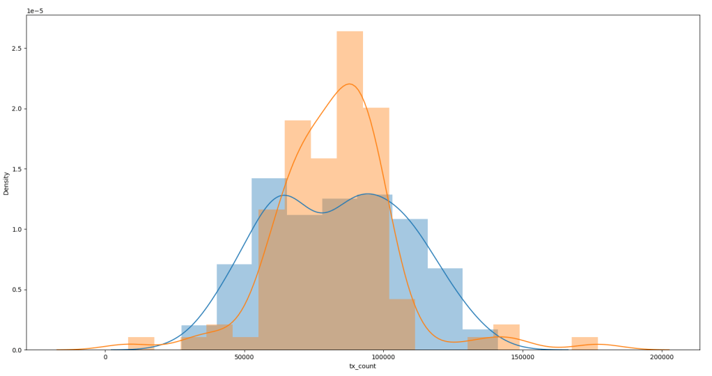
But we can see only about 340 data points available (Figure 1a) and the data is quite spiky (see Figure 1a/1b). From Figure 1 we can see the Test Data is quite Note the outliers in the historgram (Figure 1b) in the Test data. The distribution plot was produced using Seaborne (using the .distplot() method).
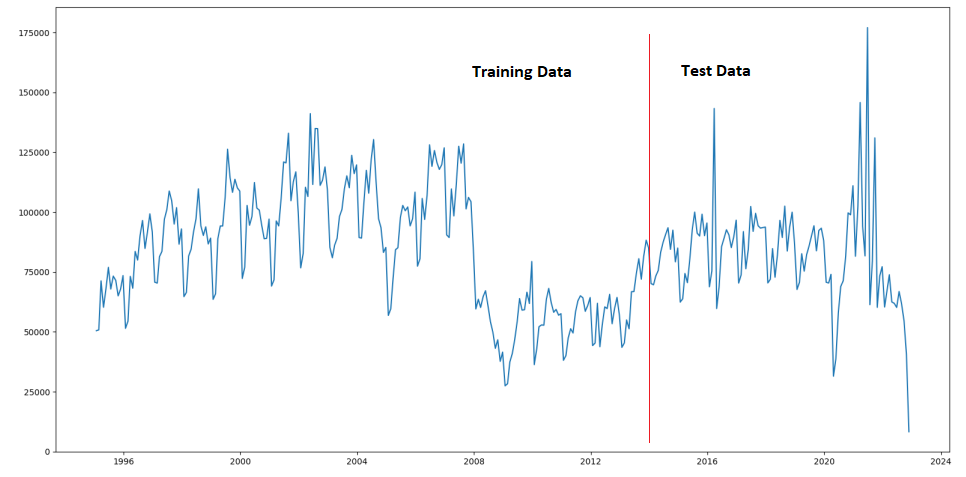
Any model that is trained on this data set is likely to not perform well especially after 2016 (see Figure 1) due to the sharp rise and fall. In fact this is the time period we would use to validate our model before attempting to forecast beyond the available time horizon.
We can see from the performance of the Neural Network (NN) trained on available data (Figure 2 Bottom) that the areas where data is spiky (orange line) the trained network (blue line) doesn’t quite reach the peaks (see boxes).

Similarly if we over sample from available data especially around the spiky regions the performance improves (Figure 2 Top). We can see the predicted spikes (blue line) are lot closer to the actual spikes in the data (orange line). If they seem ‘one step ahead’ it is because this is a ‘toy’ neural network model which has learnt to follow the last observed value.
As an aside we can see the custom Neural Network is tracking SARIMAX quite nicely except that it is not able to model the seasonal fluctuation.
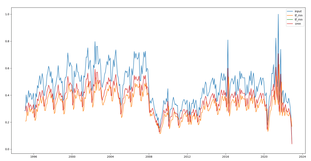
More sophisticated methods such as RNNs will product very different output. We can see in Figure 3 how RNNs model the transaction data. This is just to model the data not doing any forecasting yet. The red line in Figure 3 is a custom RNN implementation and the orange line is Tensorflow RNN implementation.
Sampling
To understand why oversampling has that effect let us understand how we sample.
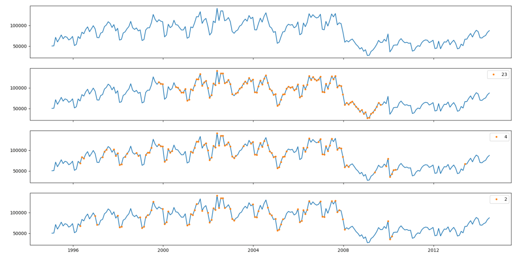
Figure 4 shows this sampling process at work. We normalise the data and take a chunk of data around a central point. For this chunk, we calculate the standard deviation. If standard deviation of the chunk is more than 0.5 the central point is accepted into the sample.
As we decrease the chunk size we see less points are collected. Smaller the chunk size more variability will be needed in the neighborhood for the central point to be sampled. For example for chunk size of two (which mean two points either side of the central point – see Figure 4), we find sampling from areas of major changes in transaction counts.
The other way of getting around this is to use a Generative AI system to create synthetic data that we can add to the sample set. The generative AI system will have to create both the time value (month-year) as well as the transaction count.
