September 2016 – Fish Eye View

Artificial Neural Networks: Training for Deep Learning – I

This is the fifth post of the series on Artificial Neural Networks and the 100th post on my blog!

To get the maximum benefit out of this post I would recommend you read the series in order, especially the post on Restricted Boltzmann Machines:

Training:

So far we have looked at some of the building blocks of a deep learning system such as activation functions, stochastic activation units (RBMs) and one-hot encoding to represent inputs and outputs.

Now we put it all together and talk about how we can train such deep networks while avoiding problems related to vanishing gradients. If you have followed the series you might have picked up the hint about using a combination of layer-by-layer training along with the traditional ‘back-prop’ based whole network training.

If not, well that is exactly what happens – usually some sort of Greedy Unsupervised Learning algorithm is applied independently (called ‘pre-training’) on each of the hidden layers, then network wide ‘fine-tuning’ is carried out using Supervised Learning methods (e.g. back-propagation).

The easiest way to understand this is to think about when you are faced with an untidy room one possible approach is to sort out things in a localised way – pick up the books, fold the clothes, tidy the bed one at a time.. this is a greedy approach – you are optimizing locally without worrying about the whole room.

Once the localised items have been sorted, you can take a look at the full room and do bits and pieces of tidying up (e.g. put stacked books on the book shelf, folded clothes in the cupboard).

Contrastive Divergence (CD) is one such method of Localised (Greedy) unsupervised learning (pre-training). We will discuss it next. It might be useful to review the post on Restricted Boltzmann Machines (see list at the top of this post) because I will use some of those concepts to illustrate the logic behind CD.

Pre-training and Contrastive Divergence (CD):

Also known as CD or CD-k where k stands for number of iterations of CD carried out (usual value is either 1 or 10 – so most often you will see CD-1 or CD-10).

Conceptually the method is simple to grasp.

We make continuous and overlapping pairs out of the input and N hidden layers (the Output Layer is excluded).
Select next pair of Layers (starting from the pairing of the Input Layer and Hidden Layer 1)
Pretend that the layer nearest to the input is the ‘visible’ layer and the other layer in the pair is the ‘hidden’ layer
Take batch of training instance and propagate them through any layers to the ‘visible’ layer of the selected pair – thereby forming a local ‘training’ batch for that pair
Update Weights using CD-k between that pair using the localised training batch
Go to Step 2

Confused as to the utility of pretending a hidden layer is a ‘visible’ layer? Don’t worry, it just gets crazier! Before we get into the details of Step 5, I want to make sure that the process around it is well understood with a ‘walk through’.

The first pair will be Input Layer and Hidden Layer 1. Input Layer (IL) is the ‘visible’ layer and the Hidden Layer 1 (HL1) is the ‘hidden’ layer.

As the Input Layer is the first layer of the network we do not need to propagate any values through. So simply present one training instance at a time and use CD (Step 5) to train the weights between IL and HL1 and the biases.

Then we select the next pair: Hidden Layer 1 and Hidden Layer 2. Here we pretend HL1 is the ‘visible’ layer and HL2 is the ‘hidden’ layer. But the training batch needs to be localised to the layer as the ‘raw’ inputs will never be presented directly to HL1 when we use the network for prediction, thus we present the training instances one at a time to the input layer, and using the weights and biases learnt in the previous iteration – propagate them to HL1 thereby creating a ‘localised’ training batch for the pair of HL1 and HL2. We again use CD (Step 5) to train.

Then we select the next pair: Hidden Layer 2 and Hidden Layer 3, create a localised training batch, use CD, move to the next pair and so on till we complete the training of all the hidden layers.

The Output Layer is excluded, so the final pairing will be of Hidden Layer N-1 and Hidden Layer N. As you might have guessed we use the global training step to train the Output Layer. It is also possible to restrict the global supervised training to just the Output Layer if that gives acceptable results.

The diagram below describes the basic procedure of pre-training.

Contrastive Divergence:

This is where things get VERY VERY interesting. If you remember from the previous post – we associate output distributions with various inputs (given the stochastic nature of RBM).

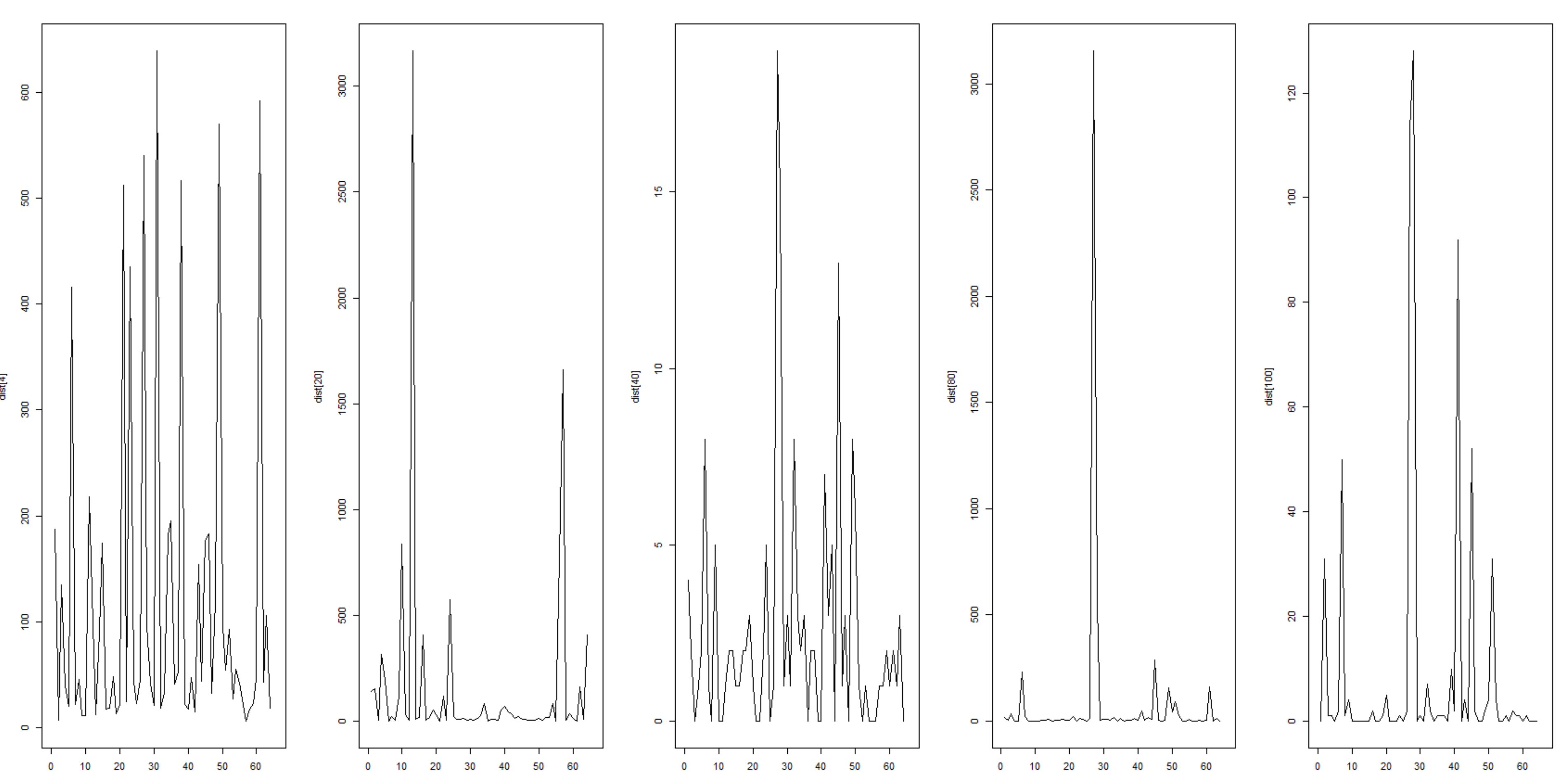
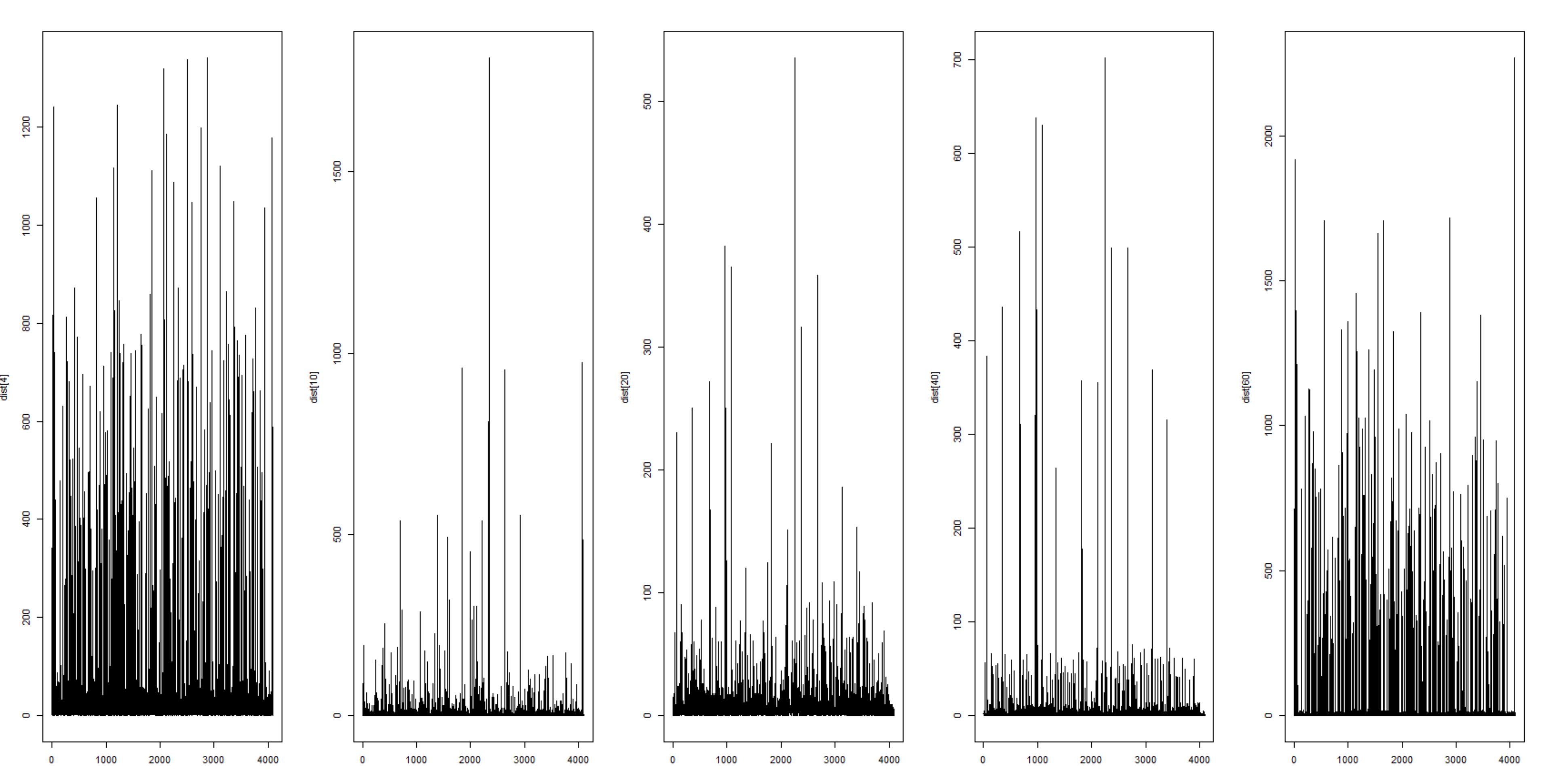
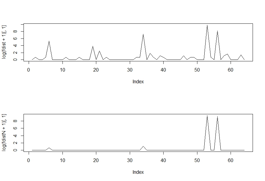
Ideally what we want is as we train a hidden layer, the distribution for the output of that layer becomes more defined and less spread out. As a limiting case we would like the output distribution to have a just one or two high probability states so that we can confidently select them as the output states associated with that input.

This is just what one would expect if we had non-stochastic output where, all other parameters remaining the same, each input is only ever associated with a single output state.

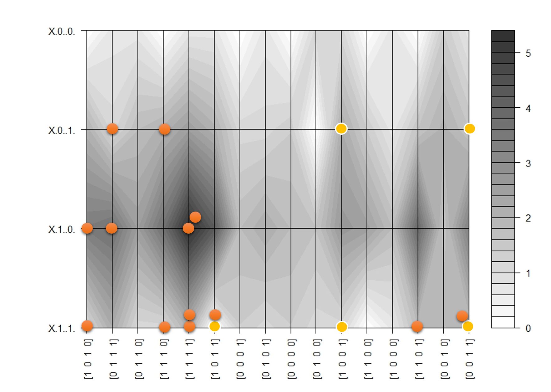
I show an example below, the two graphs are output distributions for the same input. As you might have guessed the top graph is before training and the bottom graph is after the training. These are log plots so even a small difference in the score (Y-axis) is quite significant.

Thus the central principle behind CD is that we ‘sample’ different combinations of inputs and outputs for a given set of training inputs. Using binary outputs makes sampling lot easier because we have countable, category outputs (e.g. 6 bit stochastic output = 64 possible categories). If we had a real number stochastic output then we would have potentially infinite output combinations. That said – there are examples where real number stochastic outputs are used.

At this stage because we are training a hidden layer (which we will never directly observe when the network is being used for prediction) we cannot use the corresponding output value from the training data as a guide.

The only rough guide to training we have is the fact that we need to modify the model parameters (weights and biases) in such a way that overall the high-probability associations are promoted (for the training inputs) and any ‘noise’ is removed in the final output distribution of that layer.

The approach we are taking is a ‘generative’ approach where we are seeking information about p(x, y) as compared to a ‘discriminative’ approach which seeks information about p(x | y) if x is the class label and y is the input. If you are curious about how the to approaches relate to each other and how p(x, y) can be obtained from the conditional distributions read about the

Chain Rule in Probability: p(x, y) = p(x | y) * p(y) = p(y | x) * p(x)

and the resulting

Bayes Rule: p(x | y) = p(y | x) * p(x) / p(y)

Sampling and Tuning the Model:

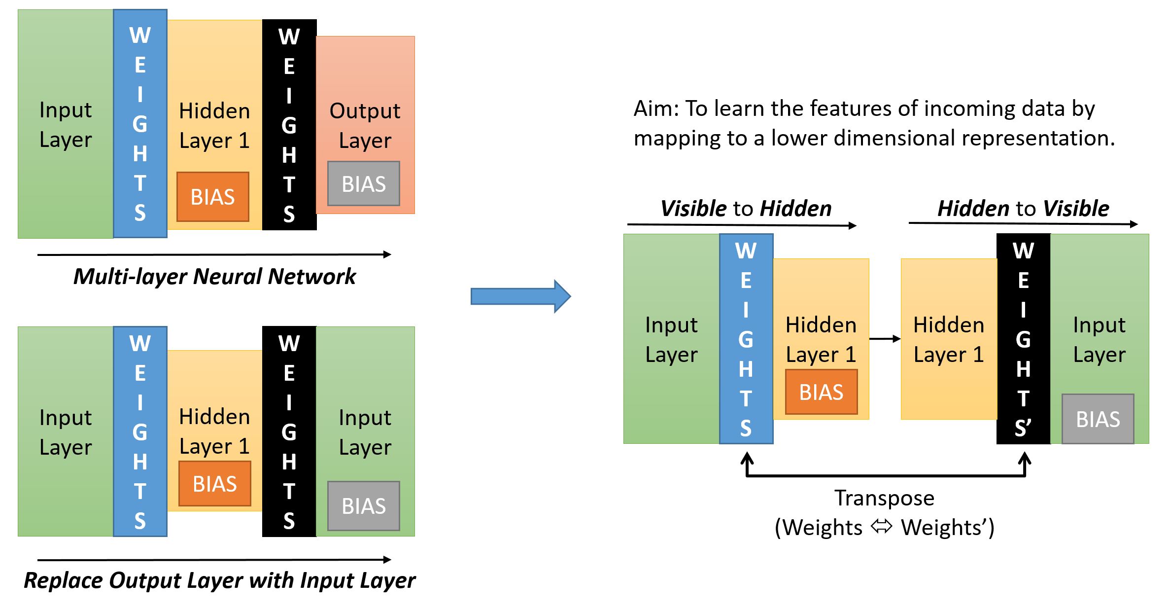
The image below describes how we collect the samples.

If we start with a normal multi-layer neural network (top left) – we find that usually the shape (in terms of number of neurons in a layer) resembles a pyramid – with the Input Layer having the maximum number of neurons and the Output Layer the minimum. The Hidden Layer is usually wider than the Output Layer but narrower than the Input Layer.

If we were to replace the Output Layer with the Input Layer (bottom left) we get a symmetric network.

To get to the layer pairing required for CD (as described previously) we just need to ensure that there is only ever one set of Weights between the paired layers (though we will have two different sets of Biases – one for Hidden Layer one for Visible Layer).

In the diagram below (on the right side) we see what the pairing would look like. In our example below the Input Layer is the visible layer and the Hidden Layer 1 is the hidden layer.

For the Sampling:

The sampling process is called ‘Gibbs Sampling’ and it involves step by step sampling from the forward and backward propagation results. See this post on Gibbs sampling for the theory behind it.

Lets keep x as the input to the visible layer and y as the output at the hidden layer. When we do the reverse propagation, following the method of Gibbs sampling, we give the output at the hidden layer back into the hidden layer – which is now the ‘visible’ layer as the input. The resulting output we get at the input layer – which is now the ‘hidden’ layer is the next value of x.

In detail:

Forward Propagation: When we propagate from visible to hidden we use the normal Weights matrix and the Bias for the Hidden Layer. I call this the forward sample – p(y|x)

Reverse Propagation: When we propagate from hidden to visible we take the transpose of the existing Weights matrix and the Bias for the Visible Layer. I call this the reverse sample – p(x|y)

We use Bernoulli Trials at both ends so our sample is always a bit string. But we also record the sigmoid output as the ‘activation’ probability for the training.

The sampling process is starts by clamping one input from our training batch, call it T[i], at the first pair of layers (Input Layer – Hidden Layer 1 – HL1). You can setup the biases for the two layers and the weights between them using a normal distribution with mean of 0 or as constant value of all zeroes.

We generate the initial y[0] value at HL1 using T[i] as the input by performing forward propagation. Call this a forward sample.
Then we take y[0], clamp it at HL1 as an input, do reverse propagation and get a reverse sample x[1].
Then we take x[1], clamp it on the Input Layer do forward propagation and get the next forward sample y[1].
Then we take y[1], clamp it at HL1 as an input, do reverse propagation and get the next reverse sample x[2].
This keeps going till we get reach the kth pair of x and y (namely x[k], y[k]). Then we use the data from the initial and kth pairs to calculate the weight and bias updates.

We then use the next input from the training batch (T[i+1]) and perform the above steps and do a weight/bias update in the end.

Weights Update:

To update the weights between the jth neuron in the visible layer and the ith neuron in the hidden layer, we use the following equation:

w[i][j] = w[i][j] + { p(H[i] = 1 | v[0]) x v[j][0] } – { p(H[i] = 1 | v[k]) x v[j][k] }

The terms in bold can be simplified as:

w[i][j] = w[i][j] + { A x B } – { C x D }

where:

A = p(H[i] = 1 | v[0]): The probability of the ith hidden layer unit to be turned on given the ‘training’ input at the visible layer at the first step of the Gibbs Sampling process.

B = v[j][0]: The sample value at the jth visible layer unit for the ‘training’ input presented

C = p(H[i] = 1 | v[k]): The probability of the ith hidden layer unit to be turned on given the kth sample of the input vector (at the kth step of the Gibbs Sampling process).

D = v[j][k]: The sample value at the jth visible layer unit for the input sampled at the kth step

A and C are basically the sigmoid outputs for the hidden layer at the start and end of the sampling process. The reason we take the sigmoid and not the Bernoulli trial result is because the sigmoid result is a probability threshold whereas the trial result is an outcome based on the probability threshold.

B and D are the initial (training) input and the final input sample obtained at the kth step of the Gibbs Sampling process.

Bias Update:

For the jth visible unit the new bias is simply given by:

b[j] = b[j] + (v[j][0] – v[j][k]) – this is same as items B and D in the weights update.

For the ith hidden unit the new bias is given by:

c[i] = c[i] + (p(H[i] = 1 | v[0]) – p(H[i] = 1 | v[k])) – this is the same as the items A and C in the weights update.

The Java code can be found here (see the Contrastive Divergence method).

The only way the weights can affect the output distribution is by modifying the probability threshold to ensure the removal of ‘noise’ from the resulting distribution. That is the only way to ‘tame’ the output distribution and link it with the input.

Once we have fully trained the current pair of layers, we move to the next pair and perform the above steps (as described before).

The idea here is to use a mini-batch of training data for CD and limiting k to a value not larger than 10 so that pairwise training of layers can proceed quickly.

This is greedy training because we are not worried about the overall effect on the network of our weight changes.

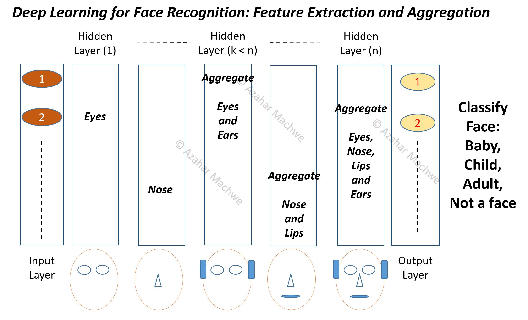
As we train the pair of layers starting from Input-HL1 pair, we are in essence learning to recognise individual features in the input data and their combinations that can help us classify one input from the other. Practically speaking at this level we are not worried about the output label, because if we can effectively distinguish between inputs using lower number of dimensions then those outputs are effectively a ‘class label’.

As a simple example of a neural network with 12 bit input layer (12 units – 4096 possible inputs), 6 bit hidden layer (6 units – 64 possible output states) and 2 bit output layer (2 units – 4 possible output states).

If we are able to, through CD-k, associate each type of the 4096 bit inputs with one of the 64 hidden unit states then effectively we have created a system that can recognise features in the input and encode for those features using a reduced dimension representation. From a 12 bit representation we are then encoding the feature space using a 6 bit representation.

Taking this reasoning to the next level, when we train the HL-1 and HL-2 pair we are learning about patterns of feature combinations one level up from the raw input. Similarly HL-2 and HL-3 pairs will learn about patterns of feature combinations two-levels up from the raw input and so on…

Why the pairing?

As a final point if you are thinking why the pairing up of layers, why not have a 3, 4, 5 layer group. The reason is if we have just two layers as a pair and we make sure the visible layer input is not the raw input but the in fact the propagated value (i.e. a localised input for that layer), then we are making sure that the output of each hidden layer unit is dependent only on the layer below. This makes the conditional probability lot simpler, if we had multiple layers we would end up with complicated conditional probability dependencies (e.g. value of Layer 4 given value of Layer 3 given value of Layer 2). In other words it makes correlation between features be only dependent on the layer below, this makes the feature correlation lot easier.

Fine Tuning:

We now need to ensure that the network is fine tuned from the Output side as we have already prioritized the Input during the pre-training.

Hint: Carrying on with the example, when we do the fine tuning training (described in the next post) our main task will be to associate the 64 hidden unit output states with one of the 4 actual output states. That is another reason why we can attempt to use normal back-prop to do the fine tuning – we do not care if the gradient vanishes as we move away from the output layer. Our main target is to train the upper layers (especially the Output Layer) to associate higher level features with labelled classes. With the CD-k we have already associated lower level inputs with a hierarchy of higher level features! With that said we can find that back-prop with its vanishing gradient problem does not give the desired results. Perhaps because our network is deep enough for the vanishing gradient problem to have a significant impact especially on training the layers closer to the Input layer. We then might have to use a more sophisticated algorithm such as the ‘up-down’ algorithm.

The diagram below gives a teaser of how the back-prop process works.

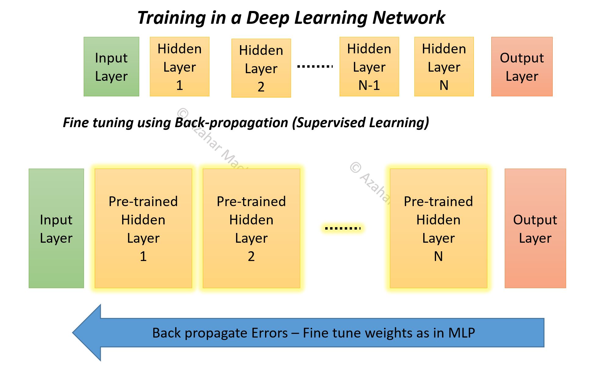
More about Fine-Tuning in the next post!

Gibbs Sampling

Gibbs Sampling is a Markov Chain Monte Carlo (MCMC) method. That sounds scary but it is really not. We are going to be using an example of neural networks to understand what Gibbs Sampling is.

Sampling is just the process of extracting information about a data set (with possibly a very large number of values) using a small sub-set of it. If the sampling is done correctly we can draw a lot of interesting conclusions about the data set given the sample.

Sampling techniques are very common: e.g. by talking to a very small sub-set of the voting population after they have given their vote (i.e. an ‘exit poll’) we are able to arrive at an estimate for the voting pattern of the entire country and an approximate idea about the final result.

Many times it is not possible to take representative samples directly or through some of the other established statistical methods (like accept-reject). There are several reasons why this could be – say we cannot directly simulate the process we want to sample from or there are almost infinitely large number of possible values.

When that is the case we can use Gibbs Sampling (if certain other conditions hold).

Monte Carlo part alludes to the fact that we use ‘repeated random sampling’ from a process which is essentially a black box due to large number of interactions going on (e.g. a neural network with large number of inputs where the outputs are tied to each other via number of hidden layers with non-linear outputs).

Given a simple 2 layer network with a visible and a hidden layer – we are roughly talking about throwing in random inputs and observing what outputs we get.

The Markov Chain part alludes to the fact that we use step by step sampling with a step size of 1 – in other words a sample obtained in step T is only dependent on the sample obtained in step T-1.

When put together the process is bit like walking blindfolded around an open space, trying to figure out its shape, with the restriction that you can only move one foot at a time where as the other foot remains grounded. The more hilly sections will allow you to take only very small steps – thus you will sample more from such regions (i.e. the high probability regions), where as in the flatter areas (low probability areas) you will be able to take much bigger steps and thus generate lesser number of samples.

To mathematically define this:

Consider a bi-variate distribution p(x, y)

We are not sure how this is generated or whether p(x, y) follows any known distribution or not.

For a neural network if we say x = input at Visible Layer and y = output at Hidden Layer, then for the MNIST example reducing the input from floating point to binary (pixel on or off) gives us 2^784 possible input values. That is a staggeringly massive number of input combinations!

For all intents and purposes – the only thing we can do is repeatedly sample two conditional distributions for a finite number of values of x and y:

p(x|y) – Probability of x given y

and

p(y|x) – Probability of y given x

The above is equivalent to taking an input value and recording the output (p(y|x)) then taking an output value and reversing the direction of propagation (by transposing the weights between visible and hidden and using the visible layer bias) and recording the ‘output’ at the visible layer (p(x|y)).

Further putting conditions imposed by Gibbs Sampling and using [t] for the current step:

Starting with initial input sample x[0] (from the training data in a neural network) – we get y[0] by propagating in the forward direction and recording the output. This is equivalent to sampling from p(y|x).

This gives us the initial values for x and y = x[0], y[0].

Then we do the ‘one foot at a time’ to start Gibbs Sampling, by keeping y = y[0] (as obtained from the previous step) and propagating in the backward direction to get the next value of x = x[1]. This is equivalent to sampling from p(x|y).

The chain therefore becomes:

x[1] ~ p(x | y[0])

y[1] ~ p(y | x[1])

………………….

x[t] ~ p(x | y[t-1])

y[t] ~ p(y | x[t])

After discarding first few pairs of x,y to allow the reduction of dependence on the initial chosen value of x = x[0] we can assume that:

x[t], y[t] ~ p(x, y)

and that the sampler is now approximately sampling from the target distribution.

Once we have a sample we can effectively investigate the nature of p(x, y).

Nature of x and y:

To be very clear, x and y may appear to be scalar values but practically speaking there is no restriction. So they can be vectors or any other entity as long as we can use them as inputs to a process and record the output. For neural networks usually x is the input vector and y is the output vector. Therefore in the generic update equations:

x[t] ~ p(x | y[t-1])

y[t] ~ p(y | x[t])

x[t] is the sample of the vector x at step ‘t’ and y[t] is the sample of the vector y at step ‘t’.

y[t] ~ p(y | x[t]) is the output of the network when we supply the vector for x that we obtained in step ‘t’ as the input

Worked Example:

Assume we have a black box network with 4 bit input (giving 16 possible inputs) and 2 bit output (giving 4 possible inputs). We can designate inputs as x and outputs as y.

We cannot examine the internal structure of the network, we have no clue as to how many layers it has or what type of units make up the layers. The only thing we can do is propagate values from input to output (giving p(y | x)) and reverse propagate from output to input (giving p(x | y)). Also we assume that the network does not change as we are sampling from it.

We follow the input clamping procedure described previously and step by step take x and y samples.

Because we are looking at 16 possible inputs and 4 possible outputs we can map the sampling process (at least the first 10 steps or so) on a contour plot where we have exhaustively mapped the joint probability between x and y:

In the contour map darker regions represent areas of high probability. The dots represent sampling path with input clamped to [1, 0,1, 1]. Yellow circles show 5 initial samples as the process ‘warms up’. Subsequent samples are concentrated around the darker areas, which means we are approximately sampling from the joint distribution.

We are not always this lucky as most real world problems do not have short binary representations. We only have the black box with inputs and outputs and some training data as a very very rough guide to how the inputs are distributed, that is why we use them as the x(0) value.

Artificial Neural Networks: Restricted Boltzmann Machines

The next building block for Deep Learning Networks is the Restricted Boltzmann Machine (RBM). We are going to use all that we have learnt so far in the ‘Building Blocks’ section (see here).

Bernoulli Trials

There is perhaps one small topic I should cover before we delve into the world of RBMs. This is the concept of a Bernoulli Trial (we have already hinted at it in the previous post). A Bernoulli Trial is an experiment (in the loosest sense) with the following properties:

There are always only 2 mutually exclusive outcomes – it is a binary result
- Coin toss – can only result in a heads OR a tails for a particular toss, there is no third option
- A team playing a game with a guaranteed result, can either win OR lose the game

The probability of both the events has a finite value (we may not know the values) which sum to 1 (because one of the two possible results must be observed after we perform the experiment)

The formulation of a Bernoulli Trial is:

P( s = 0 | 1 ) = (p^s)*(1-p)^(1- s)

If we are just interested in one of the events (say s = 1) then:

P ( s = 1 ) = p; where 0 < p < 1,

If p = 0 or 1 then it is not a probabilistic scenario – instead it becomes a deterministic scenario because we can accurately predict the result all the time (e.g.tossing a ‘fake’ Coin with two heads or two tails).

Restricted Boltzmann Machines:

A Boltzmann Machine has a set of fully connected stochastic units. A Restricted Boltzmann Machine does not have fully connected units (there are no connections between units in the same layer) but we retain the stochastic units.

When we remove the connections between units in the same layer we arrive at a now familiar structure for a feed-forward neural network. The figure above shows a simple Boltzmann Machine with 4 visible units and a RBM with 2 visible (orange) and 2 hidden units (blue).

The name Boltzmann comes from the fact that these networks learn by minimizing the Boltzmann energy of the system. In statistical physics stable systems are those that have minimum energy levels associated with the state of the different components of the system under the required constraints.

The one interesting thing that separates RBMs from normal neural networks is the stochastic nature of the units.

Taking a simple case (as done by Hinton et. al. 2006) of binary outputs (i.e. a unit is either on or off), a stochastic unit can be defined as:

“neuron-like units that make stochastic decisions about whether to be on or off”

(http://www.scholarpedia.org/article/Boltzmann_machine)

Normally (e.g. in Multi Layer Perceptrons) the activation level or score is calculated by:

summing over the incoming scores and weights only from the previous layer (the restricted part)
adding a bias term associated with the unit for which we are calculating the activation score
pushing through an activation function (e.g. sigmoid or ReLU) to get an output value

The whole system is deterministic. If you know the weights, biases and inputs you can, with 100% accuracy calculate the activation scores at each layer.

To make the system stochastic with binary output (on or off), we use the sigmoid function in step 3 (as it gives values between 0 and 1) and add a fourth step to the above:

4. use the sigmoid value as the probability score for a Bernoulli Trial to decide if the unit is on or off

As a worked example:

If sigmoid (sum(x[i]w[i][j]) + bias[j]) for jth unit is = sig[j]

Then the jth unit is on if upon choosing s uniformly distributed random number between 0 and 1 we find that its value is less than sig[j]. Otherwise it is off.

So if sig[j] = 0.56 and the random number we get is 0.42 then the unit is on with an output of 1; if the random number we get is 0.63 then the unit is off with an output value of 0.

Thus higher the sigmoid output less is the chance for the unit to be turned off, however high the value there will always be a small but finite chance that the unit is off.

Similarly lower the sigmoid output higher is the chance for the unit to be turned off, however low the value there will always be a small but finite chance that the unit is on.

This leads to something very interesting:

We end up with a ‘distribution’ of outputs for every input given the weights and biases, as compared to a deterministic approach where the output is constant for a given input as long as we do not change the parameters of the model (i.e. weights and biases).

Before we move on to an example, you might be wondering why we add this extra level of complexity? How can we ever unit-test our model? Well we can easily unit-test by setting a constant seed for our pseudo-random number generator. As to why we add this extra level of complexity, the answer is simple: It allows us to give a probabilistic result which in turn allows us to deal with errors in input patterns as well as with patterns that contradict the norm (by making the network less likely to be trapped in a local minima and to not have a difficult to change association between input and output).

This is also how our brain works. If you are familiar with hash-maps or computer memory, we need the full key / address to retrieve a piece of information (i.e. it is deterministic). Even if a single character is missing or incorrect we will not be able to retrieve the required information without a lengthy search through all the keys to find the best match (which may use some sort of a probabilistic method to measure the ‘match’).

But our brain is able to retrieve the full set of information based on small samples of itself (e.g. hearing half a dialog from a movie is enough for us to recall the full scene). This is called auto-associative memory.

Worked Example:

Assume we have a RBM with 12 input units and 6 hidden units. The units are binary stochastic type.

On the input pass the 12 inputs are passed to all the 6 hidden units (through the weighted links), bias for each hidden unit is added on, sigmoid is used followed by a Bernoulli Trial to determine if the hidden unit is on or off.

Let the input also be a binary pattern. For 12 inputs there can be at most 12 bit = 4096 possible patterns. As the output at the hidden layer is also a binary pattern we know there are finite number of them (6 bits = 64 possible patterns)

Given the stochastic nature of the hidden units, for a particular binary input pattern we are likely to see some sort of a distribution across the factorial output of the hidden layer.

We can use the finite number of possible patterns to examine the distribution for a given input and see how the network is able to distinguish between patterns based on this distribution while keeping the network parameters (weights, biases) the same.

The image above shows few plots of this distribution. Each graph is created by a single 12 bit binary input pattern.

X axis are the categorical (one of 64 possible) output patterns and Y axis the count of number of times these are seen – in each graph we keep the category (X-axis) ordering the same so that we can compare the distributions across different inputs.

These are without any kind of training (i.e. weights and biases are not updated), created by pure sampling. The distributions above allow us to distinguish between different input patterns although not with a great deal of accuracy.

We can clearly see for the input vector (1 0 1 0 0 0 0 0 0 0 0 1) – 2nd graph from left, a fairly skewed distribution with high counts towards the edges, with the max being about 3165 for output (1 1 1 0 1 0); where as for the input vector (0 0 0 0 1 0 0 0 0 1 0 0) – 1st graph from left, the counts are lower and the peaks are evenly spread out.

These distributions tell us about P(h | v) for a given W and Hb which is the probability of seeing a pattern at the hidden units (h) given an input (v) for a given set of weights from visible to hidden and Hidden Unit bias values (Hb). This is also called the ‘up’ phase.

We can also do the reverse of the above: P (v | h) for a given W’ and Vb which is the probability of seeing a pattern at the input units (v) given a hidden layer pattern (h) for a given set of weights from hidden to visible (W’ – transpose of W from above) and Visible Unit bias values (Vb). This is also called the ‘down’ phase.

Similar to the Visible to Hidden. Here each graph represents a particular pattern at the hidden layer (one of possible 64). X axis are the 4096 possible patterns we can get at the input layer when we use the transposed Weights vector and Visible Unit bias values (along with the sigmoid – Bernoulli Trial steps). Y axis is the count.

Again we see the difference in distributions allows us to distinguish between hidden values based on the frequency of resulting input values.

Next Steps:

So far we have dealt with clear cut small dimensional inputs (e.g. 2 dimensional XOR gates, 12 bit input patterns etc.) but what if we want to process a complex picture (made up of millions of pixels in this ‘megapixel’ camera age)?

In our brain because there are no deterministic links (as a very simplistic example) it is able to associate a cartoon of a car and a picture of a car with the abstract label of ‘car’. It does high level feature abstraction to enable this probabilistic mapping. We are also able to deal with a lot of error (e.g. correctly identifying a car as drawn by a child). The one disadvantage is that we may not be able to reliably recall the same piece of information all the time (like while giving an exam we are not able to recall an answer but it comes to us some point later in time).

With a probabilistic activation it would be like the 2nd from left image in the Hidden to Visible example. Where there are clearly defined peaks for certain input patterns that result when using that hidden pattern. For example when we think of a car we get associations of ‘a cartoon car’, ‘a poster of a car’, ‘the car we drive’ etc.

If it was a deterministic system we would only ever get one input pattern for a hidden pattern (unless we updated the weights/biases). The relationship (for a generic input – whether at the ‘input layer’ or ‘hidden layer’) between inputs and outputs is always one-to-one.

Note: Don’t confuse one-to-one to mean one input to one-class. One input can activate multiple classes but the point is that it will always activate the same set of classes unless we change the weights/biases.

Also even if we updated weights and biases to take into account new training data, if the association between a feature-label pair was really strong (because of multiple examples), we would not be able to modify it easily.

That brings us to the most important piece of the puzzle – how to build a network out of such layers and then train it to distinguish between even more complex patterns.

Another key point to the training is also to make the output distributions highly distinguishable and in case of multiple peaks (i.e. multiple high probability outputs) ensure all of those are relevant. As an example for predictive text we want multiple peaks (i.e. multiple probable next words) but we want all of those to be relevant (e.g. eat should have high probability next words as ‘food’, ‘dinner’, ‘lunch’ but not ‘car’ or ‘rain’).

Contrastive Divergence allows us to do just that! We cover it next time!

As usual – please point out any mistakes… and comment if you found this useful.

Artificial Neural Networks: Introduction to Deep Learning

Firstly sorry for the break! Been busy with few things. But here goes – the next instalment of our ANN series.

So far we have covered in the first and second posts:

a) To classify more complex and real world data which is not linearly separable we need more processing units, these are usually added in the Hidden Layer

b) To feed the processing units (i.e. the Hidden Layer) and to encode the input we utilise an Input Layer which has only one task – to present the input in a consistent way to the hidden layer, it will not learn or change as the network is trained.

c) To work with multiple Hidden Layer units and to encode the output properly we need an aggregation layer to collect output of the Hidden Layer, this aggregation layer is also called an Output Layer

d) The representation of the input and output can have a big influence on the performance of the neural network especially when it encounters noisy data

To the first point, while it is good to be able to add more hidden units and multiple hidden layers, we quickly come up against the problem of how to train such networks. This is not only a theoretical problem (e.g. vanishing gradient – see the first post) but also a computational one.

The Challenge:

More hidden units mean complex features can be learnt from the data
Multiple layers are difficult to train using standard back prop due to the vanishing gradient problem
Multiple layers are also difficult to train because we need to distribute the training effort so that each layer is able to support the other layers at the end of the training (a hint: perhaps we need to look at independent training of each layer to delink them?)
Adding more hidden units also increases the computational load especially if the training data set is massive, Stochastic Gradient Descent only partially solves the problem

The Solution:

Add more hidden layers (i.e. more hidden units) to make the network deeper (thus the ‘deep’ in the ‘deep learning’)
Use a combination of bottom-up and top-down learning to train this ‘deep’ network
Use specialised libraries that support GPU based distributed data processing (e.g. Tensorflow, DL4J)

Image above shows a deep learning network setup for the MNIST data set where inputs are gray-scale images (of constant pixel count 28×28) of single handwritten digits (0 to 9) which need to be mapped to their corresponding number. Each pixel in the 28×28 image is normalised and treated as an input. This gives us a full input length of 784 neurons. There are 10 digits (0 to 9) as a possible output class so the full output length is 10.

We have previously tried shallow networks and gotten good performance of about 95% with 300 hidden units organised as a single hidden layer, compare this to deep learning networks which achieve 99.7%

Deep learning works by distributing the ‘learning’ load across the hidden layers by ‘learning and aggregating’ smaller features to make larger features.

Image below shows how a Face Detector, which detects if an image contains a face of a child, baby or an adult, may distribute the feature learning and aggregation between the hidden layers.

The Building Blocks:

There are quite a few different types of ‘deep learning’ networks out there specialised for different application types (such as image tagging, document processing etc.). Some of them are not even ‘deep’ (e.g. Word2Vec) yet they incorporate novel training methods that allow them to deal with complex tasks (such as language translation) as if by magic.

I believe it will be more useful if I describe some of the common building blocks with reference to the ‘Deep Belief Network’ (Hinton et.al. 2006) as it is relatively simple (it has ‘boolean’ states in the hidden units instead of real valued ones).

The common building blocks include:

One-Hot Encoding
Softmax Layer
Sigmoid and ReLU Activation Functions
Restricted Boltzmann Machines (RBM)
Distributed Layer-wise Unsupervised Training (Contrastive Divergence)
Back-prop based Supervised Training (Fine Tuning)

One-Hot Encoding:

One-Hot Encoding is a really simple way of encoding outputs related to states.

The idea is that to represent S different states you need to have a S-bit binary string where for each state s in S only one bit in the binary string is set.

This can also be used to represent mutually exclusive classes and we have to pick one (for example a transaction cannot be both fraudulent and normal at the same time)

Let us assume we have a classifier which has to classify all inputs into one of 5 classes A, B, C, D, E.

How do we put this as an output for a neural network? Should we have just one output neuron and divide the possible output range between the 5 classes (e.g. 0-10 = Class A, 11-20 = Class B etc.), no that sounds weird especially because the output values could mean anything and nothing, also this complicates the training.

The easiest option in this case is to have one output per class, using one-hot encoding (thus a 5-bit output vector). When we train the model we simply require that the corresponding output value be significantly higher than all others so as to indicate that particular class.

One possible scheme:

A = [1,0,0,0,0]

B = [0,1,0,0,0]

C = [0,0,1,0,0]

so on..

Then if we get an output vector like:

[0.16, 0.23, 0.67, 0.03, 0.1]

we can be reasonably sure that our model is telling us the input belongs to Class C as for that class position 3 has the highest value in the label. One thing to note is that the output vector still does not tell us anything about how close two values in it are because these are just numeric values without a comparative scale (e.g. such as those found in case of probabilistic scores where all scores are compared to the value of 1 and the highest score wins).

This is where Softmax comes into the picture.

Softmax Layer:

The Softmax Layer is really straight forward to understand. It is usually found as the outermost layer of the network because it has the very important property of being able to convert ANY set of inputs into probability values such that all the values sum to 1 ( a very important property for probability values).

The softmax function is:

P(i) = e^(x(i))/Sum(e^(x(j)))

Where x(i) is the ith output that we want to convert to a probability value.

and Sum(P(i)) = 1

Below is the function in Java.

[codesyntax lang=”java”]

	/**
	 * Softmax function
	 * @param input - to be converted to probabilities
	 * @return
	 */
	public static double[] softmax(double[] input) {
		double prob[] = new double[input.length];

		double sum = 0;
		for (double val : input) {
			sum += Math.exp(val);
		}
		if (sum == 0) {
			throw new IllegalStateException("Sum cannot be zero");
		}
		for (int i = 0; i < input.length; i++) {
			prob[i] = Math.exp(input[i]) / sum;
		}

		return prob;
	}

[/codesyntax]

Example:

Assume there are 5 output units (thus length of output vector = 5) where each unit represents a class (as defined during the supervised learning phase e.g. Output Unit 1 = Class A; Output Unit 2 = Class B etc.).

For a certain input we get the following outputs (say using the Sigmoid function – see below) at Unit 1 -> 5:

[0.01, 0.23, 0.55, 0.29, 0.1]

While we can say score for Class C (Unit 3) = 0.55 looks like a good answer we cannot be 100% sure as this is not a probability value. Also Class D (Unit 4) = 0.29 is not that far off or is it? We can’t say for sure because we do not have a scale to compare against. Wouldn’t it be great if we could convert these to a probability value then we could compare them with each other and simply pick the largest value as the most probable class and ALSO provide our ‘confidence’ at the result?

If we use Softmax we get the following probability values:

[0.157, 0.195, 0.269, 0.207, 0.172]

(values are rounded to fit here so they may not exactly total to 1 – the problem with floating point arithmetic in Java)

The result is very interesting! Now we see Class C and D are just 6% away from each other (27% and 21% approx.). This is far closer than the original output vector. So while we can play it safe and choose Class C (the largest probability value) we will have to indicate somehow that we are not very sure about it as Class D came very close as well.

This can be converted to the following one-hot with a suitable confidence warning:

[0, 0, 1, 0, 0]

The interesting point about Softmax is that larger the scores, clearer is the separation between the probability values.

For example, if the output was (perhaps from ReLU units – see below):

[1, 2, 4, 3, 0]

we get probability score as: [0.032, 0.0861, 0.636, 0.234, 0.012]

This tells us there is a high probability that Class C is the correct class. The separation is now 40% between Class C and D.

Sigmoid and Rectified Linear Unit (ReLU) Activation Function:

The Sigmoid function ensures all output values are between 0 and 1. This allows us to use a probabilistic interpretation of the output. The closer the value is to 0 or 1 more confident we are about it. if the value is around 0.5 then we are not really sure.

It has the following form:

Sigmoid (x) = 1 / (1 + e^(-x))

One interesting property of the Sigmoid (which lends itself to back-prop training) is that its differential can be represented using Sigmoid:

Sigmoid'(x) = Sigmoid(x)(1-Sigmoid(x))

This also compares well with a Bernoulli Trial where Sigmoid(x) = P(x) and 1-Sigmoid(x) = Q (not x) = 1 – P(x).

This function is also used in ‘logistic regression’ where for a two class problem each class is represented by the edge values of the Sigmoid (0 and 1).

When we look at multi-class problems a common encoding follows the one-hot pattern where there is one sigmoid output per class which tells us how confident we are about that class. Remember it tells us NOTHING about how these compare with each other.

So if for 5 classes we have 5 sigmoid outputs where:

a value close to 0 means we are very sure the input does not belong to the class
a value close to 1 means we are very sure the input does belong to the class

we would still need something like a Softmax to compare these outputs with each other to choose a single class out of the 5 and reason about how confident we were about that choice.

The ReLU function comes from the behavior of a half-wave rectifier unit in electrical engineering where these units convert AC to DC. The function is VERY easy to model and process, there are no messy exponential terms. These allow just the right amount of non-linearity into a neural network thereby allowing us to handle non-linear classification tasks (more info here).

The function is:

ReLU(x) = max(0,x)

Its differential for x > 0 (required for back-prop) is a constant value of 1

The ReLU has several advantages including the fact that it is very easy to calculate and differentiate. If you see the difference it brings to the back-prop equations you will never want to even think about using Sigmoid.

The one problem with ReLUs is that once it is closed during a forward pass (i.e. x <=0) it will forever remain closed (even for backward passes). This is called the ‘dying ReLU problem’.

In the next post(s) we will cover Restricted Boltzmann Machines, Contrastive Divergence and Fine-tuning.

As usual – if I have made any mistakes do let me know!

Time-Series Dashboards with Grafana and Influx DB

I have been collecting currency data (once every hour) over the last couple of years, using a Node.JS retriever. The data goes in to a Mongo DB instance. We store the timestamp and all the currency pairings against the US Dollar (e.g. how may GBPs get you 1 USD).

Some other features we may need:

What if we want different pairings? Say we wanted to have pairings against Gold or Euros?
We may need to normalise the data if we want to compare the movement of different currencies?
We may also need ways of visualising the data (as time series etc.)

To cater to this I decided to bring in Grafana (I did not want to use the ELK stack because I believe if you don’t need text search don’t use elasticSEARCH!). Grafana does not support Mongo out of the box so I had to bring in Influx DB.

Bringing in Influx DB allowed me to integrate painlessly with Grafana (sort of). But as we all know – when you are integrating systems there is a certain minimum amount of pain you have to experience. Juggling around just shifts that pain to hopefully a location where you can deal with it efficiently. I my case I moved the pain to the integration between Mongo and Influx.

I had to create a component that pulls out the raw data from Mongo DB, pumps it through a pipeline to filter (to get the pairings of interest – the full data set has 168 currencies in it!), normalise and inject into Influx DB.

A side note: I used the Influx DB Java API which was REALLY easy to use, this encouraged me to go ahead with the Influx – Mongo integration in Java.

I also wanted the Influx – Mongo integration to be ‘on-demand’ so that we can create different pairings against different targets – such as the big 3 against Gold, major currencies against SDR (International Monetary Fund – Special Drawing Rights) etc. and populate different time-series databases in Influx. So I gave the integration a REST interface using Spark-Java.

I did encounter one problem with Grafana – InfluxDB integration was the ‘easy’ query system did not work – I had to create one manually – which is pretty straight forward as the InfluxDB documentation is decent.

Results

I was able to get the dashboards to work with normalised time-series of 6 currencies against Gold (XAU): US Dollar (USD), Indian Rupee (INR), Nigerian Naira (NGN), Euro (EUR), British Pound (GBP) and Chinese Yuan (CNY). I discovered something interesting when I was looking at the data around the ‘Brexit’ vote (23/24 June 2016).

The screenshot above is from Grafana. Filtered to show EUR-XAU, GBP-XAU, USD-XAU and NGN-XAU. We see a massive dip in Nigerian Naira before the actual Brexit vote. I was surprised so I googled and it seems that few days before Brexit vote the Naira was allowed to float against USD (earlier it was pegged to it) which led to a massive devaluation.

Then on Brexit day we see a general trend for the selected currencies to fall against Gold as it suddenly became the asset of choice once the ‘unthinkable’ had happened, with the GBP-XAU registering the largest fall. As you can see the Naira also registers a dip against Gold (XAU).

This also shows how universal Gold is. At one time all currencies were pegged against Gold, now unofficially USD is the currency of trade, but this shows when something unthinkable or truly ‘world-changing’ happens people run back to the safety of Gold.

Revisiting Apache Karaf – Custom Commands

And we are not in Kansas any more!

I wanted to talk about the new-ish Apache Karaf custom command system. Things have been made very easy using Annotations. It took me a while to get all the pieces together as most of the examples out there were using the deprecated Command system.

To create a custom command in Karaf shell we need the following:

Custom Command Class (one per Custom Command)
Entry in the Manifest to indicate that Custom Commands are present (or the correct POM entry if using maven-bundle-plugin and package type of ‘bundle’)

This is a lot simpler than before where multiple configuration settings were required to get a custom command to work.

The Custom Command Class

This is a class that contains the implementation of the command, it also contains the command definition (including the name, scope and arguments). We can also define custom ‘completers’ to allow tabbed command completion. This can be extended to provide state-based command completion (i.e. completion can adapt to what commands have been executed previously in the session).

A new instance of the Custom Command Class is spun up every time the command is executed so it is inherently thread-safe, but we have to make sure any heavy lifting is not done directly by the Custom Command Class. [see here]

Annotations

There are a few important annotations that we need to use to define our own commands:

@Command

Used to Annotate the Custom Command Class – this defines the command (name, scope etc.).

@Service

After the @Command, just before the Custom Command Class definition starts. Ensures there is a standard way of getting a reference to the custom command.

@Arguments

Within the Custom Command Class, used to define arguments for your command. This is required only if your command requires command line arguments (obviously!).

@Reference

Another optional – if your Custom Command Class requires reference to other services/beans. The important point to note here is that Custom Command Class (if you use the auto-magical way of setting it up) needs to have a default no-args constructor. You cannot do custom instantiation (or at least I was not able to find a way – please comment if you know how) by passing any beans/service refs your command may require to work. These can only be injected via the @Reference annotation. The reason for this is pretty straight forward, we want loose coupling (via interfaces) so that we can swap out the Services without having to change any config/wiring files.

Example

Let us create a simple command which takes in a top level directory location and recursively lists all the files and folders in it.

Now we want to keep the traversal logic separate and expose it as a ‘Service’ from the Custom Command Class because it is a highly re-usable function.

The listing below will declare a command to be used as:

karaf prompt> custom:listdir ‘c:\\top_level_dir\\’

[codesyntax lang=”java5″]

package custom.command;

import org.apache.karaf.shell.api.action.Action;
import org.apache.karaf.shell.api.action.Argument;
import org.apache.karaf.shell.api.action.Command;
import org.apache.karaf.shell.api.action.lifecycle.Service;

@Command(name="listdir", scope="custom", description="list all files and folders in the provided directory")
@Service
public class DirectoryListCommand implements Action
{
        //Inject our directory service to provide the listing.
	@Reference
	DirectoryService service;
	
        //Command line arguments - just one argument.
	@Arguments(index=0,name="topLevelDir", required=true, description="top level directory absolute path")
	String topLevelDirectory = null;
	
        //Creating a no-args constructor for clarity.
        public DirectoryListCommand()
        {}
        
        //Logic of the command goes here.
	@Override
	public Object execute() throws Exception
	{
		// Use the directory service we injected to get the
		// listing and print it to the console.
		
		return "Command executed";
	}
}

[/codesyntax]

The main thing in the above listing is the ‘Action’ interface which provides an ‘execute’ method to contain the logic of the command. We don’t see a ‘BundleContext’ anywhere to help us get the Service References because we use the @Reference tag and inject what we need.

This has a positive side effect of forcing us to create a Service out of the File/Directory handling functionality, thereby promoting re-use across our application. Otherwise previously we could have used the BundleActivator to initialise commands out of POJOs and register them with Karaf.

Declaring the Custom Command

To declare the presence of custom commands you need to add the following tag in the MANIFEST.MF file within the bundle:

Karaf-Commands: *

That will work for any command. Yes! it is a generic flag that you need to add in the Manifest. It tells Karaf that there are custom commands in this bundle.

Listing below is from an actual bundle:

[codesyntax lang=”text”]

Bundle-Name: nlp.digester
Bundle-SymbolicName: rd.ml.Digester
Bundle-Version: 0.0.1
Karaf-Commands: *
Export-Package: rd.ml.digester.service

[/codesyntax]